Adaptive interacting multiple model filter for AUV integrated navigation

WANG Lei, CHENG Xiang-hong, LI Shuang-xi, GAO Hai-tao

(1. School of Electrical and Electronic Engineering, Anhui Science and Technology University, Bengbu 233100, China; 2. School of Instrument Science and Engineering, Southeast University, Nanjing 210016, China)

Adaptive interacting multiple model filter for AUV integrated navigation

WANG Lei1, CHENG Xiang-hong2, LI Shuang-xi1, GAO Hai-tao1

(1. School of Electrical and Electronic Engineering, Anhui Science and Technology University, Bengbu 233100, China; 2. School of Instrument Science and Engineering, Southeast University, Nanjing 210016, China)

An improved interacting multiple model (IMM) filtering method based on expected-mode augmentation (EMA) is proposed to solve the state estimation problem for measurement noises with unknown or randomly varying statistics properties when an autonomous underwater vehicle (AUV) is in uncertain or tough environment. The proposed adaptive approach combines the expected-mode augmentation methodology and the IMM algorithm. It mainly uses the model probabilities obtained from the IMM recursive estimating process for decision making. Compared with traditional IMM algorithm, the new IMM algorithm based on EMA methodology (EMA-IMM) can capture more subtle changes of the system mode. Simulation results show that the EMA-IMM algorithm can significantly improve the precision and stability of the navigation algorithm.

autonomous underwater vehicle; integrated navigation system; interacting multiple model; expected-mode augmentation

Autonomous underwater vehicles (AUVs) are playing an increasingly important role in a number of marine applications such as weather monitoring, underwater construction, sea floor mapping and integrity check for oil pipelines under sea[1-2]. Accurate navigation systems are essential for successful operations of autonomous vehicles. For this purpose, many current researches focus on the combination of strapdown inertial navigation system (SINS) and several other auxiliary sensors such as global positioning system (GPS), Doppler velocity log (DVL), terrain aided navigation (TAN), magnetic compass (MCP). To fuse the information from the sensors, different approaches have been studied, many relying on the implementation of an extended Kalman filter (EKF)[3-4]. The performance of the EKF is reliable in many practical situations, but the nonlinear state equations may lead to instability problems. Other filtering methods can also be found in the literature, such as the unscented Kalman filter (UKF)[5-6]and the particle-based filter (PF) solution[7-8]. In most practicalapplications, the measurement noise are assumed to be Gaussian and known. However, due to the complexity of the sea conditions such as current interference, temperature variation and shifting salinities, the noise characteristics of underwater integrated navigation system usually change in the actual work environment. So an adaptive method is necessary to accommodate for changes in practical environmental conditions.

The interacting multiple model (IMM) has received much attention due to its unique power and great successes in identifying noise with unknown or randomly varying statistics properties, and in decomposing complex problems into simpler sub-problems, such as target tracking, image processing, fault detection and integrated navigation[9-11]. The general IMM algorithm, which uses a fixed set of models, usually performs reasonably well for problems with a small model set. But many practical problems involve more than just a small number of models. As a result, it is hard to get good effect when the general IMM algorithm is applied to solve those problems. However, as demonstrated by Li, it is no better to use more models addressing the same problems[12]. In recent years, variable structure multiple model (VSMM) method is proposed[13-14]. In the VSSM algorithm, the whole model space is divided into sub-model sets and the effective system model space at a certain moment can jump among those sub-model sets according to switching strategy. The switching mechanism is called Model set adaptation (MSA). The expected-mode augmentation (EMA) method is one of the mature strategies of MSA in the VSMM algorithm. The principle of EMA is to generate a set of real-time variable models named expected model from a model set of fixed structure, which is more approximate to the real mode of the system. Therefore the expected models can be used as a new model set for estimation and its corresponding results can be used to modify the estimation of fixed structure model[14]. However, VSMM algorithm is difficult to apply due to its complexity and poor real-time performance.

1 The IMM algorithm based on expected-mode augmentation method

Consider a stochastic hybrid system in which the state and measurements are dependent on the model at k moment

Where X is the state vector, Z is the observation vector, m(k) is the model state at time k, w(k, m(k)) and v(k, m(k)) are the process noise and observation noise sequence respectively. The purpose of hybrid estimation is to estimate the model and status based on all the observation time series with belt noise.

1.1 IMM algorithm

Suppose model set M, the initial Markov transition probability can be calculated at time k

Where

The model transition probability can be calculated by

The IMM algorithm can be summarized as follows:

1) Input interaction. The initial state is obtained by mixing the state estimation of all parallel filters at the previous cycle.

2) Matched model filtering. This step performs for each model an individual filtering. Therefore Kalman, extended Kalman filter, UKF, CKF or some other Gaussian filters can be applied. Then the state estimationand its corresponding estimation covariance Pj（k） can be acquired. Meanwhile, the likelihood function of each model is calculated by the Bayesian hypothesis testing method

3) Model probability update. The model transition probability can be updated as:

4) Output combination. The filter estimation based on each model is combined to generate the resulting filter state estimation according to the model transition probability.

As can be seen from the above, if the model set coincides with the real system mode, the innovation εjwill be a Gaussian white noise sequence and the model probabilities μi(k) will accurately reflect the level that associated model coincides with the real system mode.

1.2 Expected-mode augmentation method

Directed graph is utilized to clarify the relationship of filtering model set and the real system mode. Different from the general IMM algorithm in a filtering circle, at the model probability update step, model probability is utilized to generate the expected-mode E in the EMA-IMM algorithm. In the next section, EMA technical is illuminated for a hybrid system with unknown system noise.

Suppose M is a given model set of fixed structure. If there is only one uncertain parameter in the hybrid system, the grid of the model sets can be plotted with linear distribution as shown in Fig.1 (a). Each model is viewed as a grid in the mode space. An arrow from one model to another indicates a legitimate model switch with non-zero probability. The symbol “*” in the figure denotes the real system mode. It can be seen from Fig.1 that the real system mode is between m1and m3. By filtering with the fixed model set M, model probabilities associated with m1and m3will be greater than that of m2. Then, a new model set can be obtained by uniform division between m1and m3as shown in Fig.1 (b). So the expected-mode set E can be obtained which is consisted of e1, e2and e3.

Fig.1 Model set of one unknown parameter

If there are two unknown parameters in the system, the transition relations among models can be described by a plane directed graph as shown in Fig.2. It can be seen from the figure that the real system mode is in the space around by [m1, m2, m5, m6]. After filtering with the fixed model set M, the model probabilities of model m1, m2, m5and m6will be greater than other models in M. In the same way, the two dimension space around by [m1, m2, m5, m6] can be divided evenly. Then the expected-mode set E=[e1, e2,…, e9] can be used to cover the space [m1, m2, m5, m6] more detailed.

It can be seen that model probability plays an important role in decision making. That’s because it carries the information of how does the matched model coincide with the real system mode. When the number of unknown parameters in the system increases, the same manner can be used to generate the expected-mode set E. The expected-mode set E, different from original fixed structure model set M, is flexibility and variability. Models in the expected-mode set are adaptively generated from the original fixed structure model set. Obviously, models in the expected-mode set match the real system mode better than those in the fixed structure model set.1.3 The EMA-IMM algorithm

Fig.2 Model set of two unknown parameters

In the EMA-IMM algorithm, the global and local optimal estimation is considered by filtering with the fixed structure model set M and expected-mode set E. Combining the IMM estimator with the EMA methodology, the process of EMA-IMM algorithm can be summarized into following steps.

1) Fixed model re-initialization. At time k, the initial condition of each parallel filter matched with fixed model is obtained by mixing the state estimates of filters at time k-1, and the initial state, covariance matrix and model probability can be got as

2) Fixed matched model filtering. An IMM algorithm is performed with fixed structure model set M. The state estimation, covariance matrix and model probability for all the individual filters can be obtained asThen, the global estimation of filtering with fixed structure model set M, denoted as, can be got by combining all the outputs of the individual filters with weights.

3) According to the model probabilitiesthe expected-mode set E can be obtained by EMA technique.

4) Expected-mode set filtering. IMM algorithm is performed with expected-mode set E. The state estimation, covariance matrix and model probability can be obtained as. Then, the local estimation by filtering with the expected-mode set E can be obtained as

5) Estimation correcting. Using the global estimationand local estimationthe correction factor β can be calculated by

2 SINS/DVL integrated navigation system

2.1 State equation

Set the East-North-Up (ENU) frame as the navigation frame (n), Right-Front-UP (RFU) frame as the body-fixed frame (b). The state equation of the integrated navigation system is established as follows on the basis of error model of Strapdown INS and DVL:

with the state variable

Where δL, δλ are horizontal position errors; δvE, δvNare horizontal velocity errors; ϕE, ϕN, ϕUare misalignment angles; εbx, εbx, εbxare gyro constant drifts, and δvd, δΔ, δK are respectively velocity deviation error, drift angle error and scale coefficient error of DVL. W(t) and F(t) are system noises and state-transition matrix. The specific values can be found in reference[6].

2.2 System measurement equation

The observation vector is the deviation of velocity measured by SINS and DVL. As the velocity of DVL is measured in the body-fixed frame, it is necessary to be converted to the East-North-Up frame. The measurement model can be denoted as:

Where ψvis the track angle of AUV and it can be calculated by heading angle ψPand drift angle Δ.

3 Numerical simulation

Numerical simulation has been carried out to evaluate the proposed navigation solution in terms of its efficacy at integrated navigation for underwater vehicle application. The simulation conditions are as follows: the initial attitude angles are 0°, 0° and 45°, respectively. The initial latitude and longitude are 38°N and 120°E. The sampling interval is set as 0.01s. Total simulation time is set as an hour. The main parameters of the integrated navigation system are depicted as Table 1.

The measurement noise Vkis modeled by a Gaussian mixture as

Where a is a random number from the uniform distribution of [0, 1], ηkis Gaussian white noise which has zero mean and the error variance R=diag{(0.05 m/s)2, (0.05 m/s)2}.

In the simulation, the single model Kalman filter, traditional IMM filter and the proposed EMA-IMM algorithm are compared. In Kalman filter, the initial measurement noise matrix R0is set as

In the IMM and EMA-IMM algorithm, the fixed structure model set is set as

Assume the movement of the underwater vehicle including diving, surfacing and horizontal cruise, the simulated trajectory of the vehicle is shown in Fig.3.

Tab.1 Main parameters of inertial sensors

Fig.3 Trajectory for the simulated AUV

The attitude estimation errors by Kalman filter, traditional IMM and proposed EMA-IMM are illustrated in Fig.4 to Fig.6. δP, δR and δH denote the estimated error of pitch, roll and heading angle, respectively.

Fig.4 and Fig.5 depict the estimation error of horizontal angles. It can be seen that the pitch and roll estimation error decreased significantly at the beginning by all the three solutions. In Fig.6, the standard deviation of heading estimation error is obviously larger than that of the pitch and roll estimation error. The speed of convergence is slow, but all the three curves converge to certain values. This is because the observability of horizontal angles is better than that of heading angle. The results are in accord with the observability analysis presented in [15]. Meanwhile, as can be seen from Fig.6, the tracking performance of EMA-IMM is better than IMM algorithm.

Fig.4 The pitch angle error curves

Fig.5 The roll angle error curves

The horizontal velocity estimation errors by these three filtering methods are illustrated in Fig.7 and Fig.8.

It can be seen that the velocity estimates of the three algorithms converge to the value of reference. The STDs of velocity estimation error in the north direction and east direction of Kalman filter are larger than those of two other algorithms. The proposed EMA-IMM filter and IMM filter have bounded estimate errors. It can be indicated that the multiple model filters can provide a more robust estimate than Kalman filters.

The position estimation error of the three solutions are illustrated in Fig.9 and Fig.10.

They show the longitude and latitude estimation errors using the three solutions. δL and δλ are the estimated error of longitude and latitude of the vehicle’s coordinate. It can be seen that estimation by IMM and EMA-IMM are more stable than Kalman filter. The position errors of IMM and EMA-IMM algorithm grow very slowly with time. The results indicate that the performance of Kalman filter depends highly on the magnitude of the measurement noise variance. On the other hand, the multiple model filters provide betterperformance in estimation and are more stable than Kalman filter when large errors exist in the measurement values.

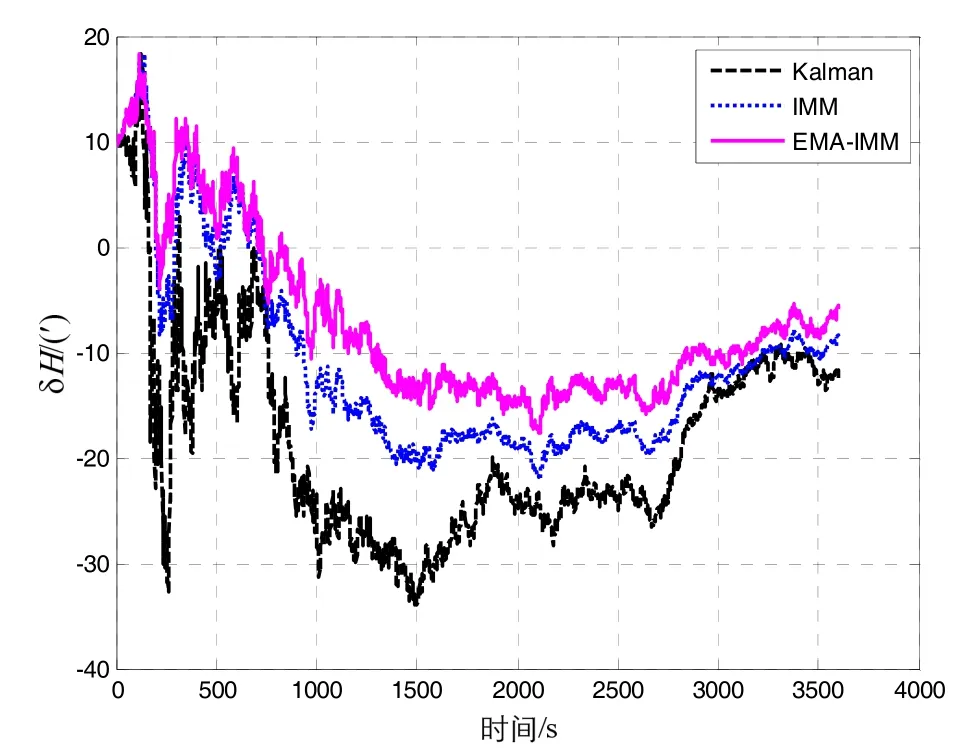
Fig.6 The heading angle error curves

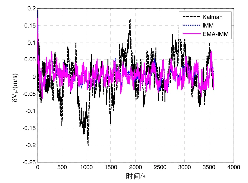
Fig.7 East velocity error curves

Fig.8 North velocity error curves

4 Conclusion

To resolve the problem when the measurement noise of the AUV integrated navigation system in the tough environment is uncertain or time-varying, an interactive multiple model filtering method based on expected-mode augmentation is proposed. Kalman filter does not have the capability of monitoring the change of parameters due to changes in vehicle dynamics. The model set of general IMM algorithm is fixed. Yet in the proposed approach, the expected-mode set can match the true noise mode well. It breaks the limitation that the structure of model set is fixed in traditional IMM algorithm. Performance comparisons on Kalman filter, traditional IMM and EMA-IMM have been conducted and the superiority of the proposed EMA-IMM algorithm has been verified in both navigational accuracy and stability.

Fig.9 The latitude error curves

Fig.10 The longitude error curves

[1] Paull C K, Caress D W, Lundsten E, et al. Anatomy of the La Jolla submarine canyon system; offshore southern California[J]. Marine Geology, 2013, 335: 16-34.

[2] Petillo S, Schmidt H. Exploiting adaptive and collaborative AUV autonomy for detection and characterization of internal waves[J]. IEEE Journal of Oceanic Engineering, 2014, 39(1): 150-164.

[3] Loebis D, Sutton R, Chudley J, et al. Adaptive tuning of a Kalman filter via fuzzy logic for an intelligent AUV navigation system[J]. Control Engineering Practice, 2004, 12(12): 1531-1539.

[4] Ndjeng A N, Gruyer D, Glaser S. Improvement of the proprioceptive-sensors based EKF and IMM localization [C]//IEEE Intelligent Transportation Systems. 2008: 900-905.

k

[5] Dawood M, Cappelle C, El Najjar M E, et al. Vehicle geo-localization based on IMM-UKF data fusion using a GPS receiver, a video camera and a 3D city model[J]. American Family Physician, 2012, 85(7): 693-700.

[6] Hui Qian, Yongzhong Ding. Research on large voyage AUV SINS/DVL combined navigation orientation precision [J]. Ordnance industry automation, 2010, 29(2): 46-48.

[7] Anonsen K B, Hagen O K. An analysis of real-time terrain aided navigation results from a HUGIN AUV[C]// Oceans. 2010: 1-9.

[8] Maki T, Matsuda T, Sakamaki T, et al. Navigation method for underwater vehicles based on mutual acoustical positioning with a single seafloor station[J]. IEEE Journal of Oceanic Engineering, 2013, 38(1): 167-177.

[9] Lee S J, Motai Y, Choi H. Tracking human motion with multichannel interacting multiple model[J]. IEEE Transactions on Industrial Informatics, 2013, 9(3): 1751-1763.

[10] Gadsden S A, Song Y, Habibi S R. Novel model-based estimators for the purposes of fault detection and diagnosis[J]. IEEE/ASME Transactions on Mechatronics, 2013, 18(4):1237-1249.

[11] Kumaradevan P, Ismail B A, Ali I, et al. Tracking endocardial motion via multiple model filtering[J]. IEEE transactions on bio-medical engineering, 2010, 57(8): 2001-10.

[12] Li X R. Multiple-model estimation with variable structure. II. Model-set adaptation[J]. IEEE Transactions on Automatic Control, 2000, 45(11): 2047-2060.

[13] Li X R, Bar-Shalom Y. Multiple-model estimation with variable structure[J]. IEEE Transactions on Automatic Control, 1996, 41(4): 478-493.

[14] Li X R, Jilkov V P, Ru J. Multiple-model estimation with variable structure - Part VI: Expected-mode augmenttation[J]. IEEE Transactions on Aerospace and Electronic Systems, 2005, 41(3): 853-867.

[15] Hong S, Man H L, Chun H H, et al. Observability of error States in GPS/INS integration[J]. IEEE Transactions on Vehicular Technology, 2005, 54(2): 731-743.

[16] 张涛, 陈立平, 石宏飞, 等. 基于 SINS/DVL 与 LBL交互辅助的 AUV 水下定位系统[J]. 中国惯性技术学报, 2015, 23(6): 769-774. Zhang Tao, Chen Li-ping, Shi Hong-fei, et al. Underwater positioning system based on SINS/DVL and LBL interactive auxiliary for AUV[J]. Journal of Chinese Inertial Technology, 2015, 23(6): 769-774.

自适应交互式多模型AUV组合导航算法

王 磊1，程向红2，李双喜1，高海涛1
（1. 安徽科技学院 电气与电子工程学院，蚌埠 233100；2. 东南大学 仪器科学与工程学院，南京 210016）

提出了一种基于期望模式修正（EMA）的改进交互式多模型（IMM）算法。该算法主要解决自主水下航行器（AUV）复杂工作环境下量测噪声统计特性未知或易发生变化时的状态估计问题，其核心思想是将期望模式修正机制和交互式多模型滤波算法相结合，利用状态估计过程中的获取的模型概率进行决策，得到更加接近与系统真实模式的期望模型集合，再通过期望模型集合滤波结果对固定模型集合滤波结果进行修正。与传统的交互式多模型算法相比，提出的基于期望模式修正的交互式多模型算法可以捕捉到系统模式更细微的变化。仿真结果表明，该算法可以大幅提高 AUV组合导航系统的估计精度和稳定性。

自主水下航行器；组合导航；交互式多模型；期望模式修正

U666.1

：A

2016-04-07；

：2016-07-27

国家自然科学基金（61374215）；安徽高校自然科学研究重点项目（KJ2016A169）；安徽科技学院人才稳定项目

王磊（1984—），男，讲师，博士，从事组合导航、多传感器信息融合方法方面的研究。E-mail: frank_408@163.com

1005-6734(2016)04-0511-06

10.13695/j.cnki.12-1222/o3.2016.04.016