A spatiotemporal evolution model of a short-circuit arc to a secondary arc based on the improved charge simulation method

Haoxi CONG (丛浩熹),Yuxuan WANG (王宇轩),Lipan QIAO (乔力盼),Wenjing SU (苏文晶) and Qingmin LI (李庆民)

State Key Laboratory of Alternate Electrical Power System with Renewable Energy Sources,North China Electric Power University,Beijing 102206,People’s Republic of China

Abstract The initial shape of the secondary arc considerably influences its subsequent shape.To establish the model for the arcing time of the secondary arc and modify the single-phase reclosing sequence,theoretical and experimental analysis of the evolution process of the short-circuit arc to the secondary arc is critical.In this study,an improved charge simulation method was used to develop the internal-space electric-field model of the short-circuit arc.The intensity of the electric field was used as an independent variable to describe the initial shape of the secondary arc.A secondary arc evolution model was developed based on this model.Moreover,the accuracy of the model was evaluated by comparison with physical experimental results.When the secondary arc current increased,the arcing time and dispersion increased.There is an overall trend of increasing arc length with increasing arcing time.Nevertheless,there is a reduction in arc length during arc ignition due to short circuits between the arc columns.Furthermore,the arcing time decreased in the range of 0°-90° as the angle between the wind direction and the x-axis increased.This work investigated the method by which short-circuit arcs evolve into secondary arcs.The results can be used to develop the secondary arc evolution model and to provide both a technical and theoretical basis for secondary arc suppression.

Keywords: short-circuit arc,secondary arc,stochasticity,improved charge simulation method,arc time

1.Introduction

Existing statistics on extra-high-voltage/ultra-high-voltage(EHV/UHV) transmission line faults have revealed that the probability of single-phase grounded short-circuit faults exceeds 90% [1,2].The secondary arc caused by singlephase grounding faults severely affects the stability and reliability of the power system.Furthermore,the spatial morphology and length of the secondary arc exhibit variations due to the stochastic nature of the transformation process from the short-circuit arc to the secondary arc [3].The arcing time of the secondary arc is severely affected as well.One of the main obstacles is that the evolution mechanism of the secondary arc is unclear.Therefore,it is paramount to study the evolution mechanism,and then provide the theoretical support for the study of the suppression methods of the secondary arc.

At present,an extremely short temporal scale and complex mechanism exist in the evolution process from the short-circuit arc to the secondary arc.Therefore,domestic and foreign scholars have limited research on this process.Despite the paucity of study on the evolution from the shortcircuit arc to the secondary arc,numerous physical experiments and simulation calculations have been conducted on the physical characteristics of the secondary arc in longdistance transmission lines.Such research provides sufficient theoretical support and an accuracy verification basis for the evolution model of the secondary arc.The physical experiment of the secondary arc is a critical method for studying its self-extinction characteristics.The extinguishing behavior of the secondary arc on EHV/UHV transmission lines has been extensively investigated in relation to the increase in voltage levels of these transmission lines [4-8].Li et al [9] established an experimental platform to study the variation of arc length as well as the motion of the arc column and arc root.Li et al [10] analyzed the reignition process during the arc duration.However,most of these studies focused on the voltammetric characteristics of the secondary arc and the arcing time,namely,ignoring the spatial form and evolution mechanism of the secondary arc.

Experiments have revealed that the arc time of the secondary arc is stochastic,and have provided considerable valid data for the subsequent study of the secondary arc.However,investigation of the evolutionary mechanism of the secondary arc from multiple perspectives is essential.With the advancement of digital computing technology,simulation calculations have become a valuable tool in compensating for the limitations of physical experiments.They provide a means to obtain crucial information regarding morphological changes,variations in arc length,and arcing time.Mathematical models have been used to calculate physical properties,such as the arc duration of the secondary arc [11-14].Tanaka et al [12] incorporated the influencing short circuit at the arc column based on the cascade chain model.This model was consistent with the motion characteristics of the arc column.Yan et al [13] used nonlinear time-variable resistance to simulate the characteristics of the secondary arc column,which supplemented the arc extinguishing criterion of the secondary arc.Liu et al [14]conducted a study on the impact of hybrid reactive power compensation (HRPC) on the arc duration.However,in the first instance,some studies failed to consider the stochasticity in the modeling procedure,resulting in the non-dispersion of arcing time.Second,the influence of thermal buoyancy was ignored when establishing the stress model of the secondary arc,which led to a longer arcing time.Moreover,the lack of the evolution procedure from the short-circuit arc to the secondary arc would have an impact on the model's degree of accuracy as well.The spatial morphology of the secondary arc is yet to be studied comprehensively.To identify the fine geometrical features of the secondary arc,image processing technology has been used to systematically process the secondary arc [15,16].The majority of these studies,however,focused only on single-image processing and excluded mechanism study.Cong et al [17] established an arc simulation model for the initial position of the secondary arc with stochasticity,which indicated that the spatial position of the secondary arc was related to the spatial conductivity and exhibited a dispersive arc time.However,the calculation conditions of the model cannot verify the influence of various conditions on the development of the secondary arc.Consequently,it is crucial to develop a spatiotemporal evolution model from the shortcircuit arc to the secondary arc with stochasticity,and to verify the accuracy in various conditions.

Based on the previous studies of gap discharges [18-20],the electric-field strength was used as the independent variable for the initiation of the secondary arc development to simulate the stochastic nature of the evolution of the secondary arc.Conventional electric-field calculation methods can be categorized into analytical and numerical methods.The complex plasma distribution within the short-circuit arc cannot be solved by analytical methods.Therefore,numerical calculation methods are used to approximate the solution.The numerical solutions for solving the electric field can be classified into two categories,namely,the field segmentation method and the boundary segmentation method [21].The long-gap discharge process can be effectively modeled using the charge simulation method,which serves as a boundary segmentation approach.This method offers the advantage of not requiring edge banding,as the electric-field strength can be directly calculated using a formula.The calculation process is straightforward,programmable,and provides a certain level of accuracy [22,23].However,the conventional charge simulation method cannot satisfy the requirements for calculating the internal electric field of the short-circuit arc,because of the tortuous spatial shape of the short-circuit arc column and the necessity to artificially create the fictitious charges.With the rapid advancement of computer technology,particle swarm optimization,genetic algorithms,annealing algorithms,and other optimization techniques have matured considerably.The efficiency of the calculation increases in terms of automatically searching for the optimal particle position when an optimization algorithm is combined with the conventional charge simulation method.Moreover,the optimization algorithm paired with the conventional charge simulation method also aims to find the global optimal solution,in addition to ensuring the memory of the three-dimensional location information and charge quantity information of fictitious charges.Particle swarm optimization is an evolutionary and self-organizing method.A major advantage of particle swarm optimization is that the algorithm includes a memory function that allows all particles to store pertinent data about the best possible solution [24].One major drawback of this algorithm is that particle swarm optimization faces the issue of convergence to the local optimal because the iterative procedure is dependent on the present optimal particle guidance.However,this issue can be solved by the improved particle swarm optimization algorithm with variable weight coefficients.Therefore,particle swarm optimization generally has a higher probability of obtaining the global optimal solution when compared to the genetic algorithm.

In this study,a model of the spatial electric field within the short-circuit arc has been developed using the charge simulation method of particle swarm optimization.The spatial electric field functions as the independent variable for the development of the secondary arc.The initial spatial form of the secondary arc is subsequently simulated by the evolution model incorporating stochasticity.

2.Model of the electric field in space inside a shortcircuit arc

2.1.Physical model of short-circuit arc

The external region of the short-circuit arc consists of air,wherein the air exhibits superior insulation properties.Due to an insufficient voltage gradient to facilitate air breakdown,the formation of an additional discharge channel within the air is not feasible.By contrast,the strong Joule heating effect produced by the large current arc of the short circuit made the surrounding air strongly ionized.Therefore,considerable free plasma exists inside the short-circuit arc channel.During the secondary arc stage,the high-conductivity free plasma did not dissipate and the air gap continued to be conductive,which made the arc discharge easier to reignite.Consequently,the secondary arc is bound to develop along the short-circuit arc channel.Numerous ions and electrons exist within the short-circuit arc channel,which renders direct calculation of the electric field inside the short-circuit arc model impossible.Therefore,the charge simulation method is used to obtain the electric-field strength in the space inside the short-circuit arc.

The conventional charge simulation method has some drawbacks because of the irregularity of the spatial shape of the short-circuit arc.First,it is challenging to pinpoint the location of the fictional charge due to the short-circuit arc's complicated form.Second,the conventional charge simulation method only reproduces the potential of a limited number of contour points on the surface of the electrode.Accordingly,a certain degree of discrete error is bound to exist.Additionally,it is necessary to perform interpolation to generate an equal number of check points at intervals along the contour points.This step is necessary for repeatedly verifying whether the fictitious charge configuration meets the accuracy requirements.Finally,the conventional charge simulation method should increase the number of contour points in complex-shaped electrodes.While rounding mistakes and digital effective bit phase reduction during the computation process increase the error,this outcome forces each column vector in the potential coefficient matrix to be excessively close to one another,creating a sick matrix [25].The identification of the fictitious charge position and quantity is the determination of the optimal solution.To avoid an increase in error caused by the aforementioned shortcomings,the conventional charge simulation method is combined with particle swarm optimization.

The cascade chain model [12] disaggregates the long gap discharge arc into several cylindrical current elements.The transition from the short-circuit arc to the secondary arc took place in the test set in [16] in 0.1 s.Consequently,this section simplifies the physical model of the short-circuit arc at 0.1 s to a large current element,which facilitates the description of the short-circuit arc space electric-field calculation model.The model in the contour point selection is displayed in figure 1.Here,101 points are uniformly considered in the arc model z-axis direction.Moreover,each point in the xoy plane is considered as the reference,in the arc boundary uniformly selecting 16 points.At the expense of some computational power,the point fictitious charge can be an excellent analog of an irregularly shaped electrode or conductor,and can replace the electrons inside the arc with discrete point charges.

After the type of fictitious charge is determined,the amount of fictitious charge also needs to be determined.The decision on how many fictitious charges to utilize should guarantee the use of fewer fictitious charges and a lower level of fitness.The fitness values calculated in the same number of iterations by three different numbers of fictitious charge are shown in figure 2.A comparison of the fitness values revealed that the fitness value was the smallest when the number of fictitious charges was 32.Therefore,32 fictitious charges are set in accordance with the calculation results shown in figure 2.Furthermore,there is no need to set separate check points when calculating the error,as the number of contour points is significantly larger than the number of fictitious charges.This approach improves the efficiency of check point settings during calculations.

The short-circuit arc obtained by applying the cascade chain model exhibits a complex curved shape.Therefore,the large current element mentioned before will be reduced to small current elements to intricately mimic the short-circuit arc.

2.2.Model based on the particle swarm optimization and charge simulation to determine the electric field in the space within a short-circuit arc

Figure 1.A schematic of contour point settings.

Figure 2.Comparison of fitness values at various fictitious charge numbers.

As the basis of model calculation,the charge simulation method is assisted by the particle swarm optimization algorithm.The key step in the calculation process is to obtain the potential coefficient matrix [P],which requires randomly initializing the position and quantity of the fictitious charge in the particles.The model solves the internal electric field of the short-circuit arc.Therefore,unlike most scenarios in which the charge simulation method is applied,the fictitious charge should be placed outside the short-circuit arc space.As a result,the fictitious charges will be dispersed at random throughout the short-circuit arc’s outer space.The radius of the short-circuit arc [17] is expressed as

where the unit of r is the meter and the unit of I is the Ampere.Here,I is the root-mean-square (rms) value.

Giving the specific quantity of fictitious charges can reduce the number of iterations.Subsequently,the particle velocity should be considerably reduced to seek optimization near the initial value,which may result in the local optimum.Therefore,the quantity of fictitious charges can be set randomly within [-1,1].

Terzija and Koglin [26] modeled the dynamic arc resistance,and revealed that the arc can be considered resistive at 0.1 s and the resistance value is certain.Namely,the standard electric potential vector [φ0] at the matching point can be derived from the experimentally measured arc voltage.Moreover,the potential at the contour point [φm] is calculated from equation (2),and the fitness value for each particle is obtained using equation (3).

where m is the number of contour points,n is the number of fictitious charges,[Pm×n] is the potential coefficient matrix,and [Qn×1] is the charge column vector.

where i is the i-th particle,m is the total number of contour points,φjis the calculated value of contour points,and φ0is the theoretical value of the j-th contour point.

Each position update of particles in the feasible domain is one iteration.At the end of each iteration,the fitness values of each particle are compared.The personal best locations Pbestare subsequently selected.The best value is selected and assigned to the global best location Gbest.The particle location update diagram is shown in figure 3.In accordance with equation (4),the particles are guided by the global best location and the personal best location until the fitness function value is satisfied or the preset number of iterations is reached.

where d=1,2,…,D,i=1,2,…,N,c1is the personal learning factor,c2is the global learning factor,both are non-negative constants c1+c2∈[0,8],and both r1and r2are random numbers between 0 and 1.

The inertia weight coefficient ω is incorporated to ensure that the last particle velocity is remembered in each iteration.In particular,the value decreases nonlinearly from 0.9 to 0.4 throughout the iterative process,as shown in equation (5).At the initial stage of the iteration,a larger inertia weight coefficient ensures that the particle velocity exhibits a superior global search capability to avoid becoming trapped in the local optimization.Furthermore,when the optimal particle range is determined,a small inertia weight coefficient ensures the local search capability and improves search efficiency.

where ωstartis the starting inertia weight coefficient,ωendis the inertia weight coefficient at the end of the iteration,and Tmaxis the maximum number of iterations.

The iterative process stops when the maximum number of iterations is reached or when the fitness value satisfies the accuracy requirement.To reduce computing space,the iterative process should stop when the fitness value satisfies the following criterion:

Figure 3.The particle position update diagram.

where Fitnessi,kis the fitness value of the k-th iteration of the i-th particle,ε is the error limit,and Smaxis the maximum number of consecutive times.

The optimal particle fitness curve,as shown in figure 4,exhibits spikes in the value of the particle fitness during the iterative process.However,the algorithm automatically adjusts to move the particles in the direction of the spatially optimal solution.The solution to the spatial electric field in the short-circuit arc channel is completed by an adapted charge simulation method,which subsequently provides the computational basis for the secondary arc evolution spatiotemporal model considering the stochasticity.

3.Spatiotemporal model for the evolution of shortcircuit arcs to secondary arcs incorporating stochasticity

3.1.Direction of the development of the secondary arc

According to the empirical formula,the arc diameter is proportional to the root-mean-square (rms) value of the arc current.The diameter of the short-circuit arc is considerably larger than the diameter of the secondary arc.Accordingly,the spatial position of the evolution of the secondary arc and the development of the short-circuit arc channel are uncertain.Therefore,the stochastic analysis should be considered in the evolution process of the short-circuit arc to the secondary arc.

The metal electrode jet electron beam only appears at the arc root position in the real evolution process.In addition,the arc root length of the secondary arc is considerably less than that of the arc column.Consequently,only the arc column’s randomness should be considered.According to the definition of an electric field E=-∇V,the higher the intensity of the electric field,the greater the spatial change rate of the potential distribution.Whereas,due to the geometrical effect of the electrode shape,the spatial variation of the potential distribution is remarkable,resulting in a large electric-field intensity.Moreover,the cathode is the arc channel’s primary electron source.As a result,the highest electron velocity and electron concentration occur at the cathode.The cathode arc root’s center functions as the secondary arc’s beginning point.

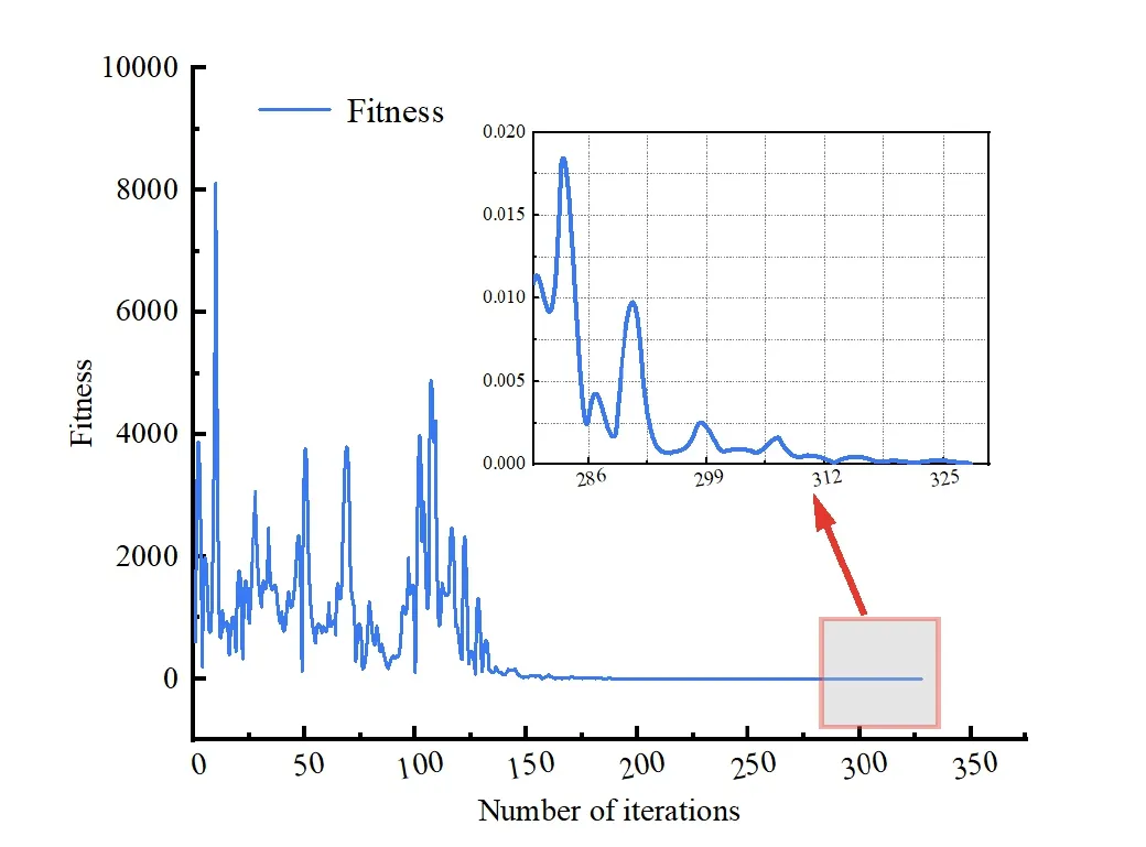
Figure 4.Fitness value curves for optimal particles based on the optimal charge simulation method.

As displayed in figure 5,in the development direction of the secondary arc,the current development point Giis considered as the center of the circle,and lstepis the upper hemispherical surface of the radius,where β is the angle between the positive direction of the z-axis and,and α is the angle between the projection of the vector xoy plane and the positive direction of the x-axis.The coordinate of the point to be developed on the aforementioned hemisphere can be derived using equation (7) by varying the values of α and β.The spatial coordinates of Giand Gi+1are shown as follows:

The stochastic representation in the evolution process is considered.According to gas discharge theory,if the field strength of the gap exceeds the gas critical breakdown field strength,the gap collapses.Because the secondary current amplitude is pretty low,it cannot satisfy the requirements for the air breakdown.Therefore,the secondary arc only evolves in the short-circuit channel.In this study,the secondary arc is more likely to form at locations with stronger electric fields.Moreover,by incorporating stochastic analysis,the probability distribution function can be obtained as follows:

where n is the number of values of angles α,m is the number of values of angles β,E(i,j) represents the magnitude of the electric field at the potential development point,and P(i,j)represents the probability that the potential development point becomes the next development point.

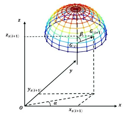
Figure 5.A diagram of the development direction of the secondaryarc.

The P(i,j) of each potential development point is an element in the probability column vector [PPmn×1],and the elements in the column vector are transformed as follows:

where Pjis the original probability column vector’s j-th element and PPiis the i-th element in the new probability column vector [PPmn×1].

The elements in [PPmn×1] are subtracted from the random number k produced by the random distribution function in[0,1] in each growth step of the secondary arc.When the difference value turns negative for the first time,the position of the element at that moment is halted,which indicates the successful position development.

3.2.Direction of the development of the secondary arc

The growth of the secondary arc stops at the anode position:namely,the forced regression of the anode arc root.Because too many plasmas are present at the anode,the development of the secondary arc cannot be separated from the electrode.The breakdown occurs between the secondary arc and the anode when the distance between the development point of the secondary arc and the anode is smaller than the critical distance ls.

where xs,ys,and zsare arc position coordinates,x,y,and z are electrode coordinates,and lsis the critical distance.

Figure 6 displays the images of the evolution from the short-circuit arc to the secondary arc under the simplified model.According to the test [16],the cathode and anode are 0.68 m apart,and the insulator is 1 m.First,the three arcs’spatial positions are very different.Second,because the three arcs are in distinct spatial positions,their arc lengths differ.The spatial configuration and arc length at the time of evolution also have an impact on the subsequent evolution of the secondary arc.

Figure 6.An evolution image of the secondary arc under the simplified short-circuit arc model.

3.3.Model calculation process

The model calculation process is displayed in figure 7.Overall,the evolution model of the short circuit to the secondary arc containing stochasticity is supported by the fictitious charge information received from the spatial electric-field model.

4.Validation of the secondary arc evolution model

The effects of the secondary arc current with various amplitudes,insulator lengths,and wind load were investigated.Moreover,the secondary arc space shape as well as arcing time was calculated to evaluate the spatiotemporal evolution model of the short-circuit arc to the secondary arc based on the improved charge simulation method.To confirm the accuracy of the model,the characteristics were contrasted with the results in the physical experiments.

4.1.Verification of arcing time dispersion under various secondary arc current amplitudes

Limited studies have been conducted on the secondary arc’s arc root.The larger the secondary arc current is,the more plasma accumulates at the arc root;thereby,the arc root extends down.Therefore,the arc root of the secondary arc is solely connected to the rms value of the secondary arc current.Here,10,30,and 50 A are the secondary arc current values,and the remaining details are listed in table 1.

The secondary arc length under three secondary arc currents is determined using the secondary arc evolution model.The box violin diagram displayed in figure 8 requires 15 valid data points for each current value to be obtained.In the violin plot,the width of the violin represents how much data is available at that arc length.Several values exist for the highest and lowest arc lengths in the 30 A and 50 A current values.Accordingly,the arc length distributions for 30 A and 50 A are flat at the lowest and highest values.

It can be seen from the data in figure 8 that the arc length under different secondary arc currents is more than 2 m,which is more than twice the discharge gap.A possible explanation for this might be that the secondary arc evolution exhibits a cascade development,similar to a lighting leader.Each step in the process of the secondary arc’s development is stochastic under the influence of the electric field.As a consequence,the arc is more tortuous.Moreover,numerous variations exist in the arc length and discreteness,under dissimilar secondary arc currents.When the secondary arc current reaches 50 A,the degree of dispersion of the secondary length is lower than those when it is under 10 and 30 A,and the median of the secondary arc length is also smaller.The transmission line parameters,which have a limited effect on the electric field in space,determine how the secondary arc current changes.The spatiotemporal model of the evolution from short-circuit arc to secondary arc considers the influence of arc roots.The arc and the electrode are connected by the cathode arc root and the anode arc root.The root length can be expressed as [27]:

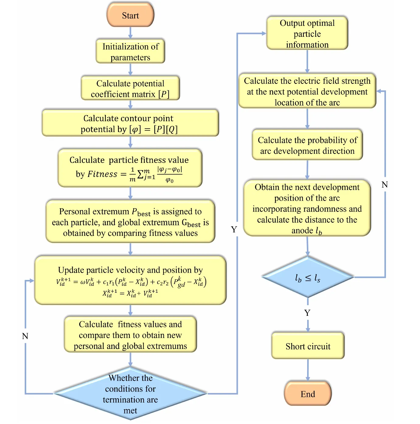
Figure 7.The calculation flow of the secondary arc evolution model.

Table 1.Parameter settings.

where kn1,kn2,kp1and kp2are all constants related to the environment.As they have little effect on the overall arc movement,the constants mentioned in equation (11) will all take mean values of their ranges in the simulation.Here,Iaand ia(t) are the root-mean-square value and instantaneous value of the arc current,respectively,lnand lpare both in units of meters,and Iaand iatake the Ampere as the unit.The length of the arc root is influenced by the effective value of the secondary arc current,with the arc root extending to a certain extent as the current increases.Therefore,in this model,the secondary arc current affects the length of the arc root,which in turn influences the secondary arc.

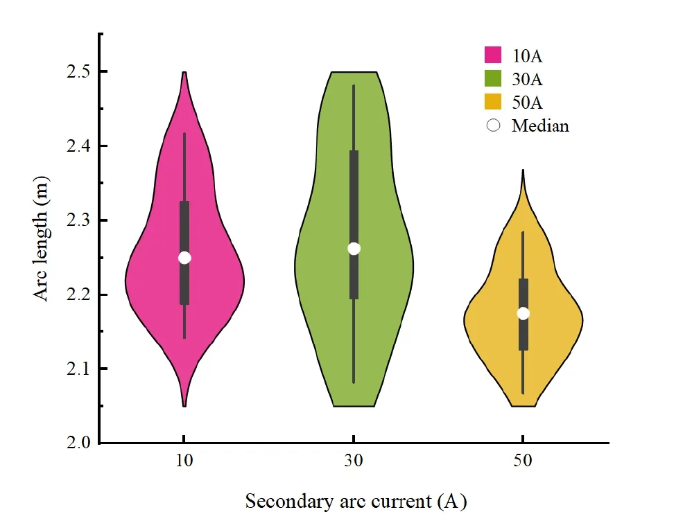
Figure 8.Arc length distributions under various secondary arc currents.

The calculation of the secondary arc burning time represents the dispersion of the arc burning time when used with the multi-field coupling cascade chain model [17].The secondary arc suffers the combined action of electromagnetic force,thermal buoyancy force,wind load and air resistance during the motion process.With the multi-field coupling cascade chain model,the force of the secondary arc can be transformed into each current element,which aids in resolving the secondary arc’s motion.The arc extinguishing condition is satisfied when the arc length is greater than the critical arc length [8],and the critical arc length fitting formula is as follows:

where the secondary arc current and recovery voltage peak values are Iamand Uam,respectively.

Calculations are performed to calculate the arcing time of an insulator with a length of 1 m and various secondary arc currents.Table 2 displays the comparison between the calculated arcing time and the test results.In general,a greater secondary current gives a longer arcing time.In lowvoltage simulation experiments,the plasma channels formed by short-circuit arcs are connected in series within the circuit.The discharge power of the circuit increases in the case where the secondary arc current increases while the power supply voltage remains constant.Therefore,the discharge energy increases with the increase in the secondary arc current,leading to an extended arc duration.However,there is stochasticity in the arc burning process of the secondary arc.Therefore,the results that deviate from the theoretical expectations are presented in table 2.As the current increases,only the minimum arc duration increases accordingly in low-voltage simulation experiments.

The error between the computed average value of the arcing time and the actual average value is the relative error of the arcing time.The relative error for various currents is 10% or less,which indicates some degree of model dependability.It is discovered that the calculated values of the arcing time are included within the measured value range in figure 9.The spatial shape and arc length of the secondary arc in the calculation model have differences when the shortcircuit arc evolves to the secondary arc.In addition,the process of subsequent evolution furthermore considers the impacts of multi-field coupling of thermal buoyancy,electromagnetic force,wind load,and air resistance.The disparities in evolutionary moments are increased because of the coupling of multiple forces.As a result,the arcing time still has dispersion,even though the secondary arc current is constant.When the secondary arc current is 30 or 50 A,the arcing time has a stronger discreteness compared to the case of 10 A.The calculated values are merely included in the randomness of the initial position,in the actual test considering the combined impacts of many factors.Therefore,the degree of dispersion of the computed values is typically minor.

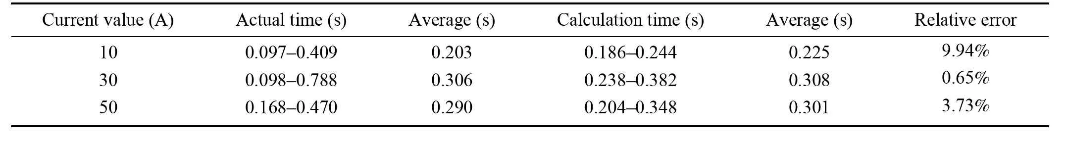
Table 2.Arcing times under various secondary arc currents.

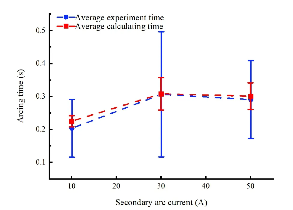
Figure 9.Arcing time dispersion.

4.2.Validation of model under various wind velocities

The wind velocity is perpendicular to the positive direction of the z-axis in three-dimensional space.In addition,the angle between the wind velocity and the positive direction of the x-axis is variable to imitate the direction of wind in nature accurately.The evolution of the secondary arc at 0.2 s is estimated using the chain arc model of multi-field coupling dynamics.The results are compared with the observed image,as shown in figure 10.First,the similarity mechanism of arc morphology can demonstrate the effectiveness of the model at the fundamental level.When a breakdown occurs,the discharge current increases abruptly,and the Lorentz force on each current element increases correspondingly.The fact that the Lorentz force is always centripetal causes the arc column to twist and spiral during the arc reignition.Consequently,the estimated 0.2 s spatial form and the spatial form of the secondary arc obtained during the physical experiment both exhibit an upward spiraling tendency.Moreover,at the quantitative characterization level,the similarity in arc diameter can also demonstrate the accuracy of the model.Since the last image in figure 10(b) is not obscured by the plasma smoke,the arc diameter can be measured.The image in figure 10(b) was processed using the method described in [16],and the resulting arc diameters at different positions were annotated in the figure.The average value of the measured arc diameters at two different positions is 1.54 cm.The secondary arc current in figure 10(a) is 30 A.According to equation (1),the arc diameter is calculated to be 1.42 cm.The error between the average measured value and the calculated value from the model is only 7.79%.Finally,the dispersion of arc duration and the relative error of the arc duration in section 4.1 both indicate that the proposed model accurately reflects the actual arc reignition process.

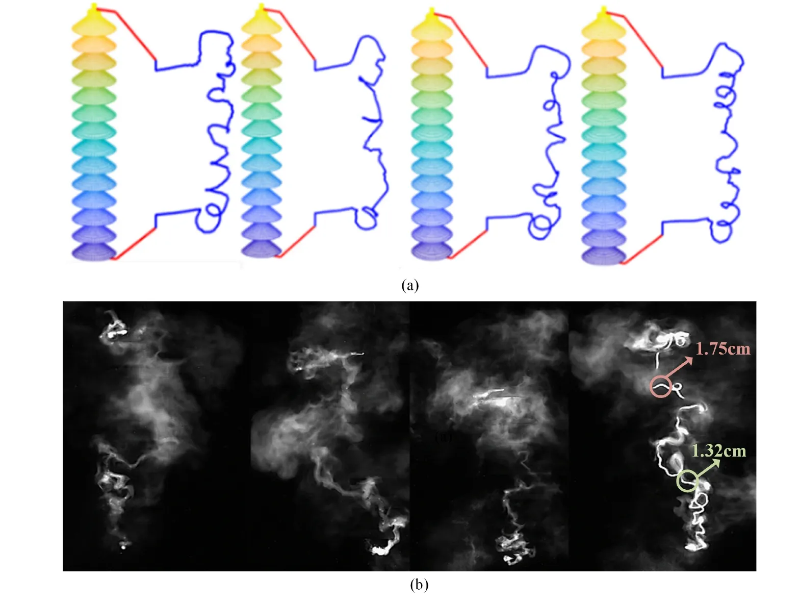
Figure 10.A comparison diagram between the calculated and measured shapes of the secondary arc at 0.2 s: (a) the spatial form of the secondary arc at 0.2 s,α=0°;(b) a physical simulation experiment image of the secondary arc at 0.2 s.

The wind velocity in figure 11 is 2.5 m s-1.The arcing time of the secondary arc tends to reduce with the increase in α.This result is consistent with the trend in a previous study[28].The arc length in the arcing time at three angles indicates various degrees of shortening.This result ties well with a previous study where,in [16],it was indicated that the arc length shortened as a result of the short circuit of the arc column during the secondary arc combustion process.

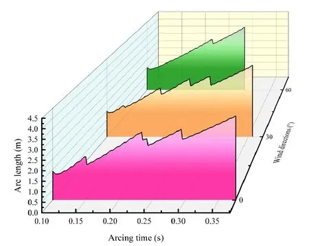
Figure 11.Arc length variation in the arcing time under various wind directions.

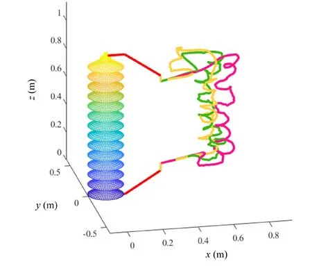
Figure 12.Spatial forms of the secondary arc under different wind speeds at 0.2 s.

When the wind velocity is 2.5 m s-1,2 m s-1or 1.5 m s-1,the secondary arc is shown by the pink line,the green line,and the yellow line,respectively,in figure 12.The only variable is the wind velocity,with no change to the other parameters.The arc extends along the x-axis significantly as the wind velocity increases.Therefore,the secondary arc’s spatial form is impacted by wind velocity as well.Wind can accelerate the deionization and thermal convection process of the secondary arc.Moreover,the arc column will be lengthened,weakening the thermal ionization degree in the arc channel.Recombination between particles is strengthened,and the difficulty of reignition is evidently increased.

4.3.Influence of the insulator length on spatiotemporal evolution process of the secondary arc

The degree of distortion of the arc column increases as thelength of the insulator increases because the thermal buoyancy effect during the development of the short-circuit arc becomes prominent.The fictitious charge distribution in the distorted component is dense and produces an electric field in the arc column to simulate the boundary conditions of the short-circuit arc channel.In addition,the distorted component is intense,and the chance that the secondary arc emerges at these points is evenly distributed,which indicates that the secondary arc distorts close to these positions.

Figure 13.The development process of the secondary arc with time under the insulator length of 1 m: (a) the development process of the secondary arc in the xoz plane;(b) the development process of the secondary arc in the yoz plane;(c) the development process of the secondary arc in the physical test.

The pressure in the arc gap decreases with the increase in the insulator length.The increase causes electrons to collide violently and stray from local thermodynamic equilibrium,namely,electrons gaining more energy.On the macro level,the arc column of the secondary arc is more tortuous.Calculations are performed to compare the development process of the secondary arc in a physical simulation experiment to the secondary arc development process over time with various insulator lengths.The results are displayed in figures 13 and 14.Figures 13(b) and 14(b) present the temporal development of the secondary arc in the yoz plane,for insulator lengths of 1 m and 1.5 m,respectively.The green and red arrows respectively represent the spatial extent of the secondary arc in the y-axis and z-axis directions.Based on the data in figures 13(b) and 14(b),it can be observed that the secondary arc exhibits minimal variations in the yoz plane.During the arc burning process of the secondary arc,it is subject to wind load in the x-axis direction and thermal buoyancy in the z-axis direction.The effect of wind load is stronger than that of thermal buoyancy.By considering both figures (a) and (b) in figure 13 and figure 14,it can be observed that as the arc burning progresses,the secondary arc undergoes noticeable variations in the x-axis direction,while its spatial position remains relatively fixed in the yoz plane.

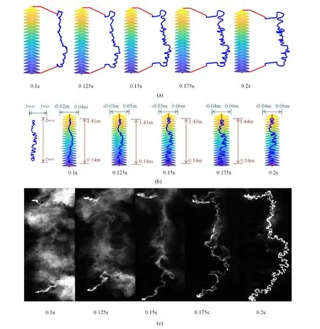
Figure 14.The development process of the secondary arc with time under the insulator length of 1.5 m: (a) the development process of the secondary arc in the xoz plane;(b) the development process of the secondary arc in the yoz plane;(c) the development process of the secondary arc in the physical test.

5.Conclusions

Based on an improved charge simulation method,the internal-space electric field of a short-circuit arc was computed.The secondary arc development model with unpredictability was created using the space electric-field model as the modeling foundation,and the secondary arc evolution process was simulated.The following are the main conclusions of the study:

(1) The spatial form of the secondary arc at 0.2 s during the evolution of the secondary arc was estimated and compared with the measured image using the stochastic secondary arc evolution model and the multi-force field coupling cascade chain model.Although the measured image shape was more distorted,the spatial form of the arc column component of the two was similar;both revealed a spiral rising spatial form.

(2) The arcing time at various secondary arc currents was calculated,and the results were compared to the measured value.The calculated value of the arcing time was within the measured value range.The arcing time and dispersion increased as the secondary arc current increased,and the average relative inaccuracy of the arcing time was within 10%.The model was reliable.

(3) The arcing time under various wind directions was determined by considering wind.As the wind increased,the arcing time shortened.Further calculations determined the variation trend of the secondary arc length during arcing time under various wind directions.The findings revealed that the measured arc lengths and those of the variation trends were similar,and that the arc length was shortened.

(4) A typical evolution process of a short-circuit arc to a secondary arc was analyzed in terms of the spatial electric field,which helps to provide a physical explanation of the phenomenon of the evolution process.On the basis of theories of dielectric strength recovery in the arc gap,the breakdown of the air gap can be understood as the effect of an electrical process.The provided model is helpful for calculating the dispersed arc duration.For instance,these results for the wind velocity,insulator length,and secondary current can help to provide guidance with regard to optimization of the single-phase-auto-reclosing scheme.

Acknowledgments

This study was supported by National Natural Science Foundation of China (Nos.92066108 and 51277061).