Life cycle greenhouse gas emissions from five contrasting rice production systems in the tropics

Pradeep K.DASH,Pratap BHATTACHARYYA,Soumya R.PADHY,Amaresh K.NAYAK,Annie POONAM and

Sangita MOHANTY

Crop Production Division,Indian Council of Agriculture Research(ICAR)-National Rice Research Institute(NRRI),Cuttack,Odisha 753006(India)

ABSTRACT Carbon footprint(CF)quantification of major rice production systems(RPSs)is a prerequisite for developing strategies for climate change mitigation in agriculture.Total life cycle greenhouse gas emissions(LC-GHGs)from rice production to consumption might provide precise CFs for RPSs.Therefore,we assessed three segments(pre-farm,on-farm,and post-farm)of LC-GHGs under five major contrasting RPSs,i.e.,aerobic rice(AR),shallow lowland rice(SLR),system of rice intensification(SRI),deep water rice(DWR),and zero-tilled direct-seeded rice(ZTR),in India to determine the corresponding CFs.Carbon footprint was the lowest for ZTR,while LC-GHGs were the lowest for AR.Therefore,AR is an adequate option for short-term reduction of GHG emissions.However,ZTR might be promoted by incentives as a long-term strategy.Among segmental LC-GHGs,on-farm GHG emissions contributed less than the other two segmental GHG emissions.The post-farm(i.e.,farm gate to consumption)segment contributed the largest proportion(54%—69%)of total LC-GHGs,followed by pre-farm(i.e.,cradle to farm)segment(21%—27%)and on-farm operation(11%—23%).These findings suggest that post-farm components that contribute to maximum GHG emissions must be scientifically tackled with proactive policy initiatives.However,the data of this segment are limited and scattered.Therefore,real-time assessment of GHG emissions during post-farm operation and input transportation from cradle to farm requires more precise quantification.Although CFin SRI was higher,this system had the potential to achieve higher yields and better soil carbon storage.Therefore,SRI may be encouraged from the perspectives of food security and long-term sustainability by reducing GHG emissions by three to four times.

KeyWords: carbon-equivalent emission,carbon footprint,climate change mitigation,global warming,management practice,soil carbon stock

INTRODUCTION

India is the second-largest rice producing country in the world,accounting for 26.9%of the total world production(FAO,2017).Rice is mainly cultivated in three ecological environments(deep lowland,shallow lowland,and upland)in India with suitable crop management practices.The major rice production systems (RPSs) in India were aerobic rice(AR),shallow lowland rice(SLR),system of rice intensification(SRI),deep water rice(DWR),and zero-tilled direct-seeded rice(ZTR).India has achieved self-sufficiency in rice production and has increased the intensity and diversity of rice-based systems in recent years(Nandanet al.,2018;Prasadet al.,2020).Rice cultivation also contributes to the global agricultural greenhouse gas(GHG)budget(IPCC,2013;Nisaret al.,2021).Starting from input production to crop growth and subsequent rice consumption,rice ecology acts as a source or sink of GHG and affects the carbon(C)footprint (CF) in agriculture.Intercultural practices (e.g.,puddling, tillage, fertilizer and pesticide application, and irrigation)in agriculture cause GHG emissions(Liuet al.,2016;Yadavet al.,2017).Furthermore,the emission patterns and their interactions with crops and soils differ from lowland to upland and among various management schemes(Pathaket al.,2012;Alamet al.,2019a;Shanget al.,2021).Innovative production technologies have been developed for rice to conserve nutrients,energy,and water(Islamet al.,2014;Dashet al.,2017)to achieve sustainable productivity and mitigate GHG emissions.However,how different RPSs drive GHG emissions and regulate CFrequires more attention for assessing the economic feasibility and environmental impacts(Gunadyet al.,2012;Bhattacharyyaet al.,2020b).

Carbon footprint is frequently used to measure the contribution of an event,process,or product to global warming.Global warming is the total CO2-C equivalent emissions across a product’s life cycle (Liuet al., 2015).Thus, CF provides specific information on each activity and directs a course of action to reduce emissions(Finkbeiner,2009;Liuet al., 2015).Carbon footprint is a widely accepted and precise indicator in the agricultural sector to judge the efficacy of a system from climate change perspective(Lowet al.,2016;Xueet al.,2018).Moreover,it is a quantitative indicator of GHG emissions that is useful for identifying eco-friendly production systems and developing strategies for climate change mitigation(Pandey and Agrawal,2014;Rezaeiet al., 2021).Furthermore, the assessment of life cycle GHG emissions(LC-GHGs)is an acceptable approach for assessing CFin different sectors,including agriculture(Brocket al., 2012; Jianget al., 2020).Specific knowledge regarding how different management practices regulate GHG emissions in rice through LC-GHGs is imperative.The assessment of LC-GHGs accounts for all segments of a product(system basis),including resources utilized,processes involved,and transportation of products from the site of generation to the site of consumption,waste generated,etc.(Arvanitoyannis,2008;Soheili-Fardet al.,2018).Life cycle assessment(LCA)commences with the acquisition of raw materials from natural sources(earth)to make a specific product and ceases with the return of all materials associated with that product to nature.It evaluates all aspects of a product’s life cycle with the idea that they are interrelated(Royet al.,2009).The assessment of LC-GHGs in agriculture provides valuable information on pollutants,soil acidification,groundwater contamination,GHG emissions,and eutrophication(Finkbeineret al.,2006;Pathaket al.,2012;Jainet al.,2013;Alamet al.,2019a).A comprehensive examination of LC-GHGs and CFs of various RPSs can provide information about the environmental consequences of the technologies used and the required management strategies(Yadavet al.,2018).

Therefore, the specific objective of our study was to quantify the CFs in five contrasting RPSs through comprehensive assessment of LC-GHGs to identify the mitigation options associated with GHG emissions.This quantification will help in policy making for climate change mitigation by both public and private organizations.

MATERIALS AND METHODS

Studysite and soil C determination

This study was conducted at the National Rice Research Institute(NRRI)in Cuttack,which is situated in the eastern part of India(20◦44′N,85◦94′E,24 m above mean sea level).The experimental site has a tropical climate,with an annual average precipitation of approximately 1 500 mm and the monsoon prevalent from June to October.The soil texture is sandy clay loam and is categorized as Aeric Endoaquept.The RPSs,viz.,AR,SLR,SRI,DWR,and ZTR,were maintained with four replications in their respective ecological niches.The cropping history of the experimental plots consisted in rice followed by rice/fallow.Rice(c.v.Oryza sativaL.)varieties Apo,Gayatri,Swarna,Varsha Dhan,and Pooja were transplanted/sown in line (the spacing between rows and between hills within rows were 20 and 15 cm,respectively)(Table I).The recommended dosage of chemical fertilizer was applied as prescribed for the region to the respective systems.Urea was used as the source of nitrogen and was administered at three split doses,50%as basal and 50%as two top-dressings(25%each).Single basal doses of potassium and phosphorus were applied as potassium chloride and single superphosphate,respectively.Standard recommended techniques were used for insect,disease,and weed controls(Table I).

The wet digestion method was used to measure soil total organic C(TOC)content.Concentrated acids(concentratedH2SO4:85%H3PO4=3:2)were used in the digestion block,which was heated to 120◦C for 2 h(Snyder and Trofymow,1984).The mass of TOC(MTOC,Mg ha-1)was estimated by multiplying TOC(g kg-1)by bulk density(BD,Mg m-3)and soil depth(Depth,m).Therefore,MTOC in the topsoil layer(0—30 cm)was estimated as per Eq.1(Pathaket al.,2011):

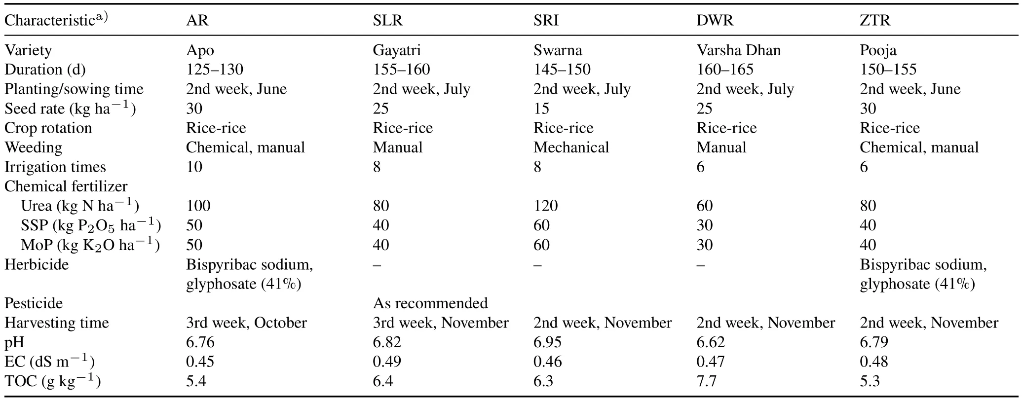
TABLE I Characteristics of five major contrasting rice production systems,i.e.,aerobic rice(AR),shallow lowland rice(SLR),system of rice intensification(SRI),deep water rice(DWR),and zero-tilled direct-seeded rice(ZTR),in India

Soil C stock was estimated based on the difference between final and initial MTOC in the surface soil(0—30 cm)under different production systems(Eq.2).Initial TOC data were obtained during the initial year of each cropping system(2008—2009).

GHG emissions

Gas samples for CH4and N2O estimation were collected continuously during the crop growing season at approximately 5—7 d intervals in each system using the closedchamber technique.The chamber was 53 cm× 37 cm×71 cm(length×width×height)in size(Bhattacharyyaet al.,2013a;Dashet al.,2017).Aluminum base plates were inserted into the soil in all systems during sowing/transplanting and were kept in the field until harvest.To measure CH4and N2O fluxes,six rice hills were taken within the chamber placed on the base plate.The air within the chamber was thoroughly mixed using a battery-operated fan,and gas samples were collected in a Tedlar gas sampling bag(M/s AeroVironment Inc.,Arlington,USA).Gas sampling was performed using a 50-mL plastic syringe with a hypodermic needle(24 gauge)at two different instances with an interval of 30 min and was measured during 9:00 a.m.to 11:00 a.m.(Zhanget al.,2012;Bhattacharyyaet al.,2014).Gas chromatography(TRACE 1110,M/s Thermo Fisher Scientific Pvt.Ltd.,Nasik,India),consisting of flame ionization detector,electron capture detector,and Porapak Q column(stainless steel,1/8-inch thick in outer-diameter,80/100 mesh size, and 6 feet long for CH4and 13 feet long for N2O),was used to measure the relative concentrations of CH4and N2O.Successive linear interpolation techniques were used to fill the gap in CH4and N2O fluxes(mg m-2h-1)when sampling was not performed(Dashet al.,2017).Cumulative CH4and N2O emissions(kg ha-1)during crop production in the field were estimated by the summation of daily fluxes throughout the crop growing period.

where ∆XCH4and ∆XN2Oare the difference of CH4and N2O concentrations, respectively, between two different instances with an interval of 30 min,EBVSTP(L)is the effective chamber volume at standard temperature and pressure,t(min) is the time interval between initial and final gas sampling,andA(m2)is the surface area of the chamber.

Global warming potential(GWP)refers to the cumulative radiative forcing of all GHGs at a fixed time scale,keeping CO2-equivalent(CO2-eq)emissions at unity,i.e.,at a value of 1(IPCC,2013).This helps to account for the relative potential of a particular GHG to trap and radiate back longwave radiation(heat)to the atmosphere,compared to CO2.Global warming potential(t CO2-eq ha-1)was estimated according to the IPCC guideline for a 100-year time horizon(IPCC,2013;Xiaet al.,2016;Shanget al.,2021).

Carbon-equivalent(C-eq)emissions(CEE,t C-eq ha-1)and greenhouse gas intensity(GHGI,t C-eq t-1)were estimated using the following equations(Bhattacharyyaet al.,2012;Dashet al.,2017):

LC-GHGs in RPSs

The LC-GHGs were adopted to estimate CFby considering GHG emissions from rice cradle to consumption stages(Lal,2004;Pathaket al.,2012;Alamet al.,2019a)under five contrasting RPSs.Four important steps were followed for LCA:1)definition of the goal,2)creation of a life cycle inventory, 3) impact assessment, and 4) interpretation of the results.The LCA principles and methods were used to assess CFin terms of tons of C emissions per ton of rice production(Alamet al.,2016;Shanget al.,2021).The CF values were estimated by subtracting soil C stock from the total LC-GHGs in RPS.

Establishing goal and defining scope.The fluxes of GHGs linked to different components in RPSs were estimated based on specific crop management practices(Table I).The system boundary for each RPS was fixed up to consumption,dividing into pre-farm(i.e.,cradle to farm),on-farm, and post-farm (i.e., farm gate to consumption)segments(Fig.1).We used the C emissions(derived from total LC-GHGs)per ton of rice production in each system as a functional unit.The life cycle inventory was built based on the mass-balance technique,considering the contribution of all inputs and outputs per ton of rice yield in the fixed system boundary.The GHG emissions during pre-farm activities were determined using emission factors and the quantity of each input used for their production, processing, and transportation to the field.While the GHG emissions during on-farm operations included the use of farm implements,machinery,chemicals,manual labor,etc.,the GHG emissions resulting from farm gate to consumption were associated with cleaning,soaking,steaming,drying,steel hull milling,transportation,packaging,marketing,and final consumption(Table II).The net C emissions in each RPS per ton of rice production were estimated by the summation of emissions from all three segments(pre-farm,on-farm,and post-farm)(Fig.1).

Fig.1 Approaches for analysis of life cycle greenhouse gas emissions(LC-GHGs)in rice production systems(RPSs).The system boundary for each RPS was fixed up to consumption,dividing into pre-farm(i.e.,cradle to farm),on-farm,and post-farm(i.e.,farm gate to consumption)segments.

Life cycle inventory.Life cycle inventories were created with the factors driving rice yield(e.g.,seeds,chemical fertilizers,chemicals for plant protection,machinery,fuel,electricity,and manual labor).The GHG emissions were estimated from the emission factors for manufacturing,transport,and utilization of inputs as well as outputs.Soil GHG(CH4and N2O)fluxes were considered as the positive side of soil emissions,while soil C stock was considered as the negative side in each system(Table II).In this study,we considered soil CO2emission neutral,considering it as a biogenic source within the system, where photosynthesis and respiration,along with decomposition,take place simultaneously at an approximately similar rate(IPCC,2013).

Pre-farm GHG emissions.Activities that contribute to GHG emissions during the production and transport(supply)of inputs to the farm gate were considered for calculation of GHG emissions.Indirect emissions due to manufacturing of chemicals and farm machinery(Table II)were estimated through life cycle inventories(Lal,2004;Pathaket al.,2012;Alamet al., 2019a).The cost of manufacturing farm machinery(as a functional unit)was calculated by multiplying the emission factors of each machinery production(0.15 kg CO2-eq US$-1) by72.44 Indian rupees (United States dollar-Indian rupee exchange rate on April 17,2021).

Emissions associated with the transportation of inputs for production were obtained from published literatures(Lal,2004;Pathaket al.,2012;Alamet al.,2019a).Transportation through the sea(trans-oceanic bulk cargo carrier)and lightduty diesel trucks (3—7 t capacity taken with an average mileage of 4 km per liter)for road transport were considered.The transportation of inputs from the factory to the farm gate that accounts for GHG emissions is represented as ton-kilometers(t-km)for travelling by road and ton-nautical miles(t-nm)for travelling by sea.The weight of each input was multiplied by the distance travelled from experimental fields to input source to obtain t-km or t-nm (Lal, 2004;Alamet al.,2016;Zhenget al.,2017).

On-farm GHG emissions.On-farm GHG emissions begin with land preparation in each production system.The estimates included emissions during land preparation(fuel of power tiller),sowing/transplanting,application of chemicals,fertilizers,and pesticides,weeding,irrigation(electricity for water pumps), other intercultural operations, and harvesting.A power tiller was used for land preparation in four production systems(excluding zero tillage).In those systems,manual labor was considered for sowing and transplanting.Fuel consumption by farm machinery was estimated by considering land area,liters of fuel consumed per hectare,time taken for the operation,and the frequency of operationin each production system(Alamet al.,2019a;Shanget al.,2021).The emission factors of electricity consumed by 3HP irrigation pump(≤2.3 kW)were estimated(Lal,2004)and these values were used to estimate CEEs.Manual labor(manhour ha-1)was considered based on the actual man-hours used(in the study)for each production system to produce one ton of rice yield.The GHG emissions in the rice fields were directly measured from each production system through the manual closed-chamber method.

Post-farm GHG emissions.The activities contributing to GHG emissions from farm gate up to consumption were considered post-farm components.These included cleaning,soaking,steaming,drying,steel huller,milling,transportation up to 500 km,packaging,marketing,and other activities(Pathaket al.,2012).

Total LC-GHGs and CF.The data inventory of inputs and outputs (Table II) was multiplied by the respective emission factors(Table III)to obtain total CO2-eq emissions(i.e.,sum of pre-farm,on-farm,and post-farm emissions)for each RPS.Lastly,CO2-eq emissions were further converted into CEEs.The CF(t C-eq t-1)in each RPS was obtained by subtracting soil C stock in the 0—30 cm topsoil layer from the total LC-GHGs in each system(Alamet al.,2019a).

Statistical analysis

The GHG emissions per ton of rice production,inputs required for cradle to farm, farm to farm gate, and farm gate to consumption,net and total GHG emissions,and soil C stock were statistically analyzed using SAAS 9.2 online version.The mean and standard deviation of each system were compared and Duncan’s multiple range test(DMRT)was performed.

RESULTS

Soil GHG emissions,GWP,CEE,GHGI,and rice yield

The CH4fluxes during the crop growing period varied from 0.32 to 1.64,0.54 to 4.07,0.42 to 4.01,0.80 to 5.53,and 0.14 to 3.70 mg m-2h-1, in AR, SLR, SRI, DWR,and ZTR,respectively(Fig.2).Meanwhile,cumulative CH4fluxes varied among the systems(Table IV):DWR had the highest seasonal cumulative CH4emission(115.1 kg ha-1),while AR had the lowest cumulative CH4emissions(34.5 kg ha-1).

The N2O fluxes during the crop growing period ranged from 19.6 to 55.9, 9.1 to 38.7, 4.0 to 38.7, 3.4 to 34.8,and 5.1 to 34.8µg m-2h-1in AR,SLR,SRI,DWR,and ZTR,respectively(Fig.2).As shown in Table IV,the highest seasonal cumulative N2O emissions were observed in AR(1.40 kg ha-1),followed by SRI(1.10 kg ha-1),SLR(1.03 kg ha-1),ZT(0.91 kg ha-1),and DWR(0.86 kg ha-1).

Among the RPSs tested,DWR showed the highest estimated seasonal mean GWP(3.92 t CO2-eq ha-1),whereas AR showed the lowest(1.48 t CO2-eq ha-1).The CEE values were estimated for all the RPSs and ranged from 0.40 to 1.07 t C-eq ha-1with the ranking of DWR>SLR>SRI> ZTR> AR.Specifically, DWR showed a significantly higher CEE than any other system.Yield-scaled C emissions or GHGI was significantly higher in DWR than in any other system and followed the same pattern as GWP and CEE.Significant variation in grain yield was observed among the systems.It ranged from 4.19 to 6.05 t ha-1and was the highest in SRI and the lowest in DWR.

LC-GHGs and CFs

Crop management practices of RPSs significantly altered LC-GHGs,which decreased in the following order of SRI>SLR>ZTR>DWR>AR.Total LC-GHGs for one ton of rice production were 1.18,1.11,1.04,1.06,and 0.94 t C-eqt-1in SRI,SLR,ZTR,DWR,and AR,respectively(Fig.3).Specifically, AR showed the lowest CEEs among the five production systems.

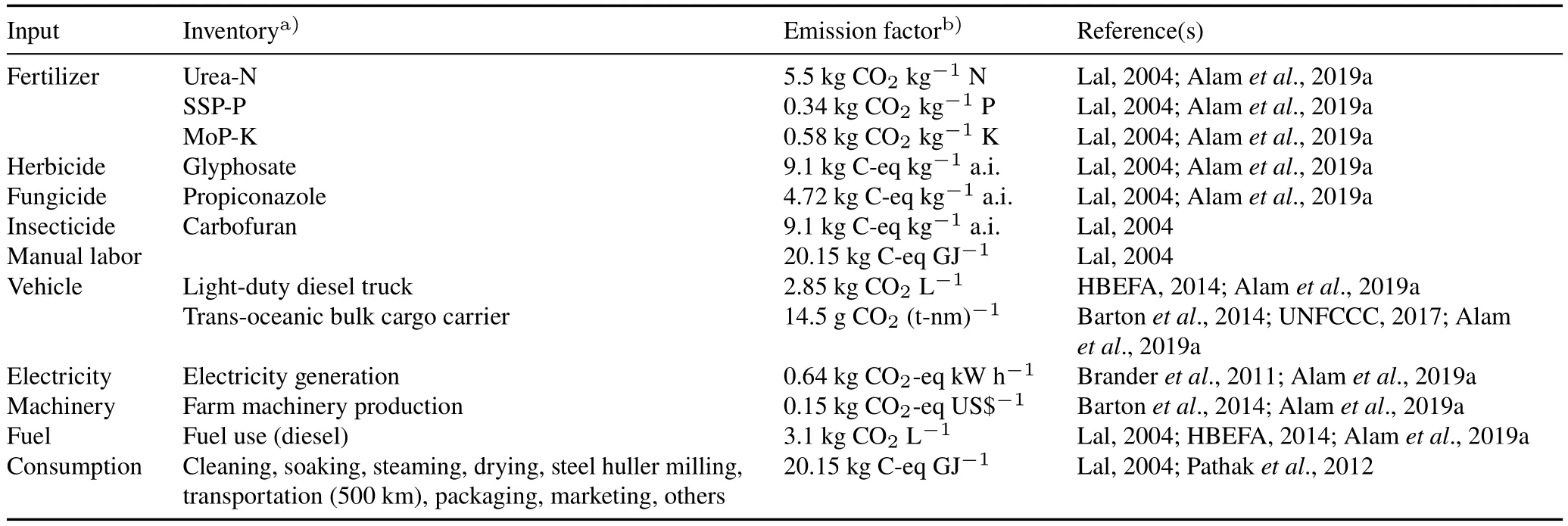
TABLE III Input and output data sources and their emission factors for rice cultivation under five different systems

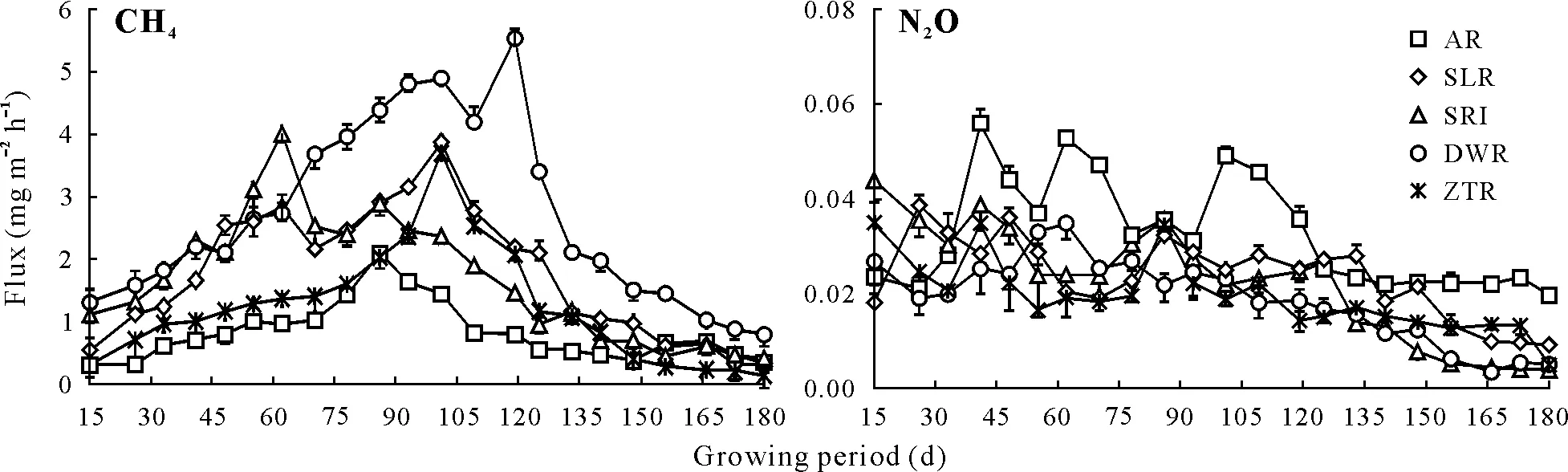
Fig.2 Soil CH4 and N2O fluxes during the growing period under five major contrasting rice production systems,i.e.,aerobic rice(AR),shallow lowland rice(SLR),system of rice intensification(SRI),deep water rice(DWR),and zero-tilled direct-seeded rice(ZTR),in India.Vertical bars indicate standard deviations of the means(n=4).

TABLE IV Soil CH4 and N2O emissions,global warming potential(GWP),C-equivalent(C-eq)emission(CEE),greenhouse gas intensity(GHGI),and rice yield(RY)under five major contrasting rice production systems(RPSs),i.e.,aerobic rice(AR),shallow lowland rice(SLR),system of rice intensification(SRI),deep water rice(DWR),and zero-tilled direct-seeded rice(ZTR),in India

Fig.3 Total life cycle greenhouse gas emissions(LC-GHGs)and carbon footprints(CFs)for one ton of rice production in five major contrasting rice production systems,i.e.,aerobic rice(AR),shallow lowland rice(SLR),system of rice intensification(SRI),deep water rice(DWR),and zero-tilled direct-seeded rice(ZTR),in India.Vertical bars indicate standard deviations of the means(n=4).Bars with the same letter are not significantly different at P ≤0.05 among rice production systems.C-eq=C-equivalent.

Pre-farm GHG emissions per ton of rice production were 0.26, 0.24, 0.24, 0.23, and 0.23 t C-eq t-1for AR, ZTR,SRI, SLR, and DWR, respectively, and were higher than on-farm emissions(Fig.4).Pre-farm GHG emissions were the lowest in SLR and the highest in AR,and were 9.9%,2.2%,0.5%,and 1.3%higher in AR,SRI,DWR,and ZTR,respectively, than in SLR.In the context of aerobic rice cultivation,chemical application and manufacturing(fertilizer, herbicide, fungicide, and insecticide)accounted for a higher proportion of total CO2-eq emissions during the prefarm stage.Transportation of commodities and agricultural equipment contributed the most to GHG emissions at the pre-farm boundary,accounting for 37.2%in AR,27.2%in SLR, 25.4% in SRI, 30.2% in DWR, and 28.9% in ZTR(Fig.5).

On-farm GHG emissions were considerably lower than pre-farm and post-farm GHG emissions.Among the RPSs,AR showed the lowest LC-GHGs for one ton of rice production(Fig.4).

Fig.4 Life cycle greenhouse gas emissions(LC-GHGs)under different segments for one ton of rice production in five major contrasting rice production systems,i.e.,aerobic rice(AR),shallow lowland rice(SLR),system of rice intensification(SRI),deep water rice(DWR),and zero-tilled direct-seeded rice(ZTR),in India.Vertical bars indicate standard deviations of the means(n=4).Bars with the same letter are not significantly different at P ≤0.05 among rice production systems.C-eq=C-equivalent.

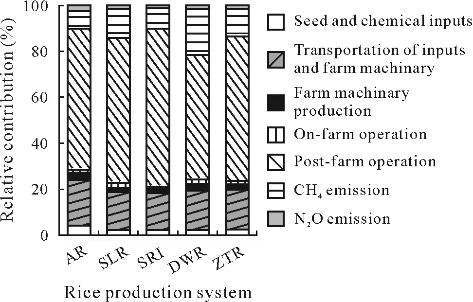
Fig.5 Relative contributions of different components to net life cycle greenhouse gas emissions in five major contrasting rice production systems,i.e.,aerobic rice(AR),shallow lowland rice(SLR),system of rice intensification(SRI),deep water rice(DWR),and zero-tilled direct-seeded rice(ZTR),in India.

After farm gate,rice reaches consumers through various post-farm processes,which emit mostly CO2.The energy consumption in each post-farm process contributed to their corresponding C emissions.Thus,LC-GHGs in post-farm processes were 0.81,0.70,0.67,0.57,and 0.56 t C-eq t-1in SRI,SLR,ZTR,AR,and DWR,respectively(Fig.4).

The relative contributions of components to LC-GHGs varied among the production systems.Irrespective of different components,post-farm operation contributed the maximum proportion to total LC-GHGs,followed by transportation of inputs and farm machinery and then soil emissions(Fig.5).

Soil C stock and CF

Soil C stock in the five RPSs ranged from 0.41 to 1.9 t ha-1,decreasing in the following order of ZTR>SRI>SLR>DWR>AR.The CFper ton of rice production among the tested production systems varied from 0.57 to 0.87 t C-eq t-1and the lowest value was found in ZTR and the highest value in SRI.The ZTR system saved 28.3%,34.0%,48.6%,and 53.3%CEEs per ton of rice production over DWR,AR,SLR,and SRI,respectively(Fig.3).Therefore, the CFto produce one ton of rice production followed the order of ZTR

Total LC-GHGs

Total LC-GHGs were assessed holistically for five RPSs in India using three segments: i) pre-farm (i.e., cradle to farm),ii)on-farm,and iii)post-farm(farm gate to consumption) (Alamet al., 2019a).A similar method was applied by other researchers for LCA of pre-farm segment in rice,rice-vegetable, and rice-wheat systems (Takiet al., 2018;Alamet al., 2019a; Harunet al., 2021).We adopted the methodology recommended by Pathaket al.(2012) and Jainet al.(2013)to quantify GHG emissions in post-farm segment,which includes threshing,cleaning,milling,processing,storing,and consumption.Secondary data were used to assess the LCA in post-farm segment in our study,which is representative of the lower Gangetic Plain of India.However,we believe that an elaborate and exhaustive site-specific database may provide a better estimation (Venkat, 2012;Ghasempour,2018;Xuet al.,2020).We estimated the transportation cost of input supply to farm gate on a real database considering the distances of factory outlets and mode of transportation(Xueet al.,2014;Singhet al.,2020).Emission factors were used to convert GHG emissions to CEEs for input production.Emission factors of input production were obtained from published literatures(Soamet al.,2017;Alamet al., 2019b).To make the estimation uniform and easy to understand,we converted all emissions into GWP and CEEs per ton of rice production.A similar approach was recently used by researchers for CFanalysis (Yadavet al.,2018;Mohammadiet al.,2020).Emissions for input production,transportation,and consumption were equal for different RPSs,as all were tested on the same experimental farm.However,GHG emissions per ton of rice production varied due to the variations in grain yield among the systems.

The assessment of LC-GHGs is an important approach for environmental impact assessment across different sectors including agriculture(Brocket al.,2012;Jainet al.,2013).In recent years,the assessment of LC-GHGs has been applied in the areas of agriculture and food production to improve the environmental efficiency of production chains(Gillaniet al.,2010).In our study,the assessment of LC-GHGs in five RPSs was relevant because of differences in irrigation patterns, fertilizer management, and tillage schemes.The major advantage of this method is that we can compare different RPSs in a common platform to devise mitigation options for climate change.The difficulty in the assessment of LC-GHGs in different RPSs is ecological variance that sometimes masks the effect of specific management practices.

We measured the on-farm GHG emissions in each system and converted them to CEEs per ton of rice production.In our study, aerobic rice emitted less gas than the other systems.Energy consumption was relatively low because puddling,transplanting,and continuous flooding conditions were not practiced(Saberet al.,2020;Chenet al.,2021).On the other hand,SRI and SLR showed higher on-farm GHG emissions,basically due to puddling,transplanting,higher organic matter addition, and maintenance of continuous flooding conditions in the field(Habibet al.,2019; Saberet al.,2020;Chenet al.,2021).Few options are available to reduce GHG emissions in deep-water rice systems(Gathorne-Hardy,2013).It is an ecologically stressed system in which fertilizer and water management are difficult(Houshyar and Grundmann, 2017; Yodkhumet al., 2017).However, adjusting planting time and introducing smart fertilizers could effectively reduce on-farm GHG (particularly N2O) emissions in deep-water rice(Bhattacharyyaet al.,2013b;Phonget al.,2021;Raimondiet al.,2021).Zero-tilled direct-seeded rice yielded relatively less but sequestered more C in soil and emitted less GHGs (Nuneset al., 2017; Alamet al.,2019b).Higher C stock in ZTR might be due to crop residue addition(Prechslet al.,2017;Saberet al.,2020)and a lower rate of soil C decomposition,as soil disturbance decreased(Alamet al.,2019a;Saberet al.,2020).Relatively higher CH4emissions were recorded in SRI and SLR due to continuous submergence conditions and increased addition of organic matter, which is supported by our previous work(Bhattacharyyaet al.,2012,2013a)and the findings of other researchers(Agnese and Othman,2019;Yadav Set al.,2020;Derooet al.,2021).In SRI and SLR,N2O emissions were lower than in AR,where alternate wetting and drying prevailed(Nelsonet al.,2015;Setyantoet al.,2018;Tirol-Padreet al.,2018).In AR and ZTR,puddling,transplanting,and continuous water stagnation were not practiced,resulting in a lower GWP and reduced emissions,and then lower CFs.These two systems might be promoted from the perspective of climate change mitigation with certain incentives in terms of input or compensation,as rice yield might be lower in the first year of cultivation(Pathaket al.,2011; Parthasarathiet al.,2012;Mangalasseryet al.,2015;Bhattacharyyaet al.,2020a;Yadav Set al.,2020).

CFs

The CFis the mirror of a C-efficient green system.We estimated CFbased on total LC-GHGs in each production system counterbalanced by soil C stock.This is a precise CFanalysis method that can be replicated in various production systems with site-specific modifications(Goglioet al.,2018;Alamet al.,2019a;Yadav G Set al.,2020).Assessment of LC-GHGs is a well-accepted tool for analyzing and estimating CEEs for GHG emissions (Lal, 2004; Pathaket al., 2012; Bartonet al., 2014; Alamet al., 2019a, b).We found the smallest CFin ZTR,compared with the other four RPSs.This was primarily due to lower GHG emissions and a higher soil C stock(Alamet al., 2019b; Guardiaet al.,2019;Arunratet al.,2021;Zhanget al.,2021).Therefore,this should be promoted from the perspective of longterm environmental sustainability.On the other hand,AR contributed the least to total LC-GHGs,indicating the possibility of climate change mitigation.However,because of the low C stock potential,the CFof this system was higher than that of ZTR.Therefore,AR can be recommended for the immediate reduction of GHGs on a short-term basis.Moreover,better residue or organic C management practices can enhance the C stock potential in AR (Rahmanet al.,2019; Mahmood and Gheewala,2020; Saberet al.,2020;Yadav Set al.,2020).Therefore,AR may be promoted in a large area of irrigated rice ecology in India and Southeast Asia(Tirol-Padreet al., 2018; Alamet al., 2019a; Yadav Set al., 2020).The CFs of SRI and SLR were higher in our study, indicating that they are not as environmentally friendly as the other three systems(Pathaket al.,2011;Xueet al., 2018; Yadav G Set al., 2020).However, from the perspective of food security and higher productivity,these two systems are worthy of implementation in developing countries (Hossain and Majumder, 2018; Sapkotaet al.,2019;Aryalet al.,2020).Therefore,enhanced management of nitrogen and water resources in these systems can be adopted to mitigate or reduce on-farm GHG emissions two to three times(Bhattacharyyaet al.,2020a,b).Mid-season drainage and real-time nitrogen management using a customized leaf color chart,SPAD,or a sensor-based approach might effectively reduce GHG emissions in SRI and SLR.

CONCLUSIONS

The CFwas lower in ZTR, whereas it was higher in SRI.However,total LC-GHGs were lower and CFwas higher in AR compared to ZTR,as soil C stock was smaller.Therefore, if we focus on short-term or immediate GHG emission reduction,AR seems to be a good option.However,for a long-term strategy, ZTR with lower CFand higher soil C stock potential should be promoted with incentives.Segment-wise LC-GHGs revealed that post-farm segment contributed the maximum(54%—69%)to total LC-GHGs,followed by pre-farm(21%—27%)and on-farm(11%—23%)segments.These findings suggest that post-farm components that contribute to GHG emissions need to be carefully addressed with proper infrastructure development and policy initiatives.Production and transportation of inputs require site-specific distribution and an efficient mode of transportation.However,although on-farm GHG emissions are frequently quantified,they contributed to a relatively lower amount of GHG emissions,compared to the other two segments.The precise real-time assessment of GHG emissions during post-farm processes and transportation of inputs from cradle to farm requires more quantification,as the data of those two segments are limited and scattered.Although CF was higher for SRI,this system showed a potentially higher yield and sequestered more C in soil.Thus,in view of food security,SRI could make more energy efficient and should be promoted in developing countries,by reducing emissions by 30%—40%in postharvest handling of the product.

ACKNOWLEDGEMENTS

This work was supported by the Indian Council of Agriculture Research(ICAR)-National Fellow Project(No.Edn./27/08/NF/2017-HRD;EAP-248),the ICAR-National Innovations in Climate Resilient Agriculture Project(No.EAP-245), the Department of Biotechnology(DBT),Governmen of India(No.BT/PR25417/NER/95/1185/2017),and the National Rice Research Institute(NRRI).The authors heartedly appreciate the assistance and direction provided by the Director of the ICAR-NRRI.