Finite element analysis of an all-steel buckling-restrained brace

Jiang Tao ,Dai Junwu ,Yang Yongqiang ,Bai Wen ,Pang Hui and Liu Rongheng

1. Key Laboratory of Earthquake Engineering and Engineering Vibration,Institute of Engineering Mechanics,China Earthquake Administration,Harbin 150080,China

2.Key Laboratory of Earthquake Disaster Mitigation,Ministry of Emergency Management,Harbin 150080,China

Abstract: Typical all-steel buckling-restrained braces (BRBs) usually exhibit obvious local buckling,which is attributed to the lack of longitudinal restraint to the rectangle core plate.To address this issue,all-steel BRBs are proposed,in which two T-shaped steel plates are adopted as the minor restraint elements to restrain the core plate instead of infilled concrete or mortar.In order to investigate the factors that characterize the hysterical responses of this device,different finite element (FE)models are developed for the specific context.The FE models are developed based on nonlinear finite element software,which incorporate continuum (shell or brick) elements,large displacement,and deformation formulations.In these FE models,two different steel constitutive models are adopted to precisely reproduce the cyclic response of the BRB component.Meanwhile,comparisons between the numerical and experimental results are conducted to validate the effectiveness and accuracy of the robust FE model.The agreements between experimental observations and numerical predictions demonstrate that the FE method could be utilized for in depth parametric analysis.Furthermore,BRBs with detailed configurations can provide excellent hysteretic behavior and seismic performance through the optimal design process.

Keywords: steel BRB;T-shaped steel;finite element model;optimal design;hysteretic behavior

1 Introduction

Buckling-restrained braces (BRBs) were first developed in Japan in the 1980s (Wakabayashiet al.,1973) and gained popularity in the United States after the Northridge earthquake in 1994.Due to their unique configurations,BRBs can survive large axial compressive load without any premature buckling,when compared with ordinary steel braces.Furthermore,BRBs exhibit a nominally symmetric cyclic response with strain hardening under uniaxial loading,and the corresponding force-displacement curves are stable and ample.Thus,buckling-restrained braces have been widely used worldwide as ductile seismic-proof members in seismic zones.

Although there are many variations of geometric configurations of BRBs in practical applications,the fundamental energy dissipation mechanisms are the same.A typical BRB is composed of a ductile steel core(the yielding element,hereafter called the “core”),which is designed to yield in both tension and compression.To preclude global buckling,the core is usually wrapped with a steel casing,which is subsequently filled with mortar or concrete.Before casting mortar into the casing,an unbounded material or a very small air gap between the core and mortar is provided to minimize,or eliminate,if possible,the transfer of axial force generated by the core to the mortar and the steel casing.Considering Poisson′s effect,this small gap between the core and the mortar is also needed to allow for the core′s free expansion.

Since the early development of BRBs,different materials and configurations have been fully studied through full-scale and small-scale experiments.The first tests were conducted in Japan (Wakabayashiet al.,1973),which were followed by Kimuraet al.(1976).After the Northridge earthquake,the development of this device was started in the USA based on a large number of experimental tests (Blacket al.,2002;Merrittet al.,2003;Sunet al.,2019;Pandikkadavath and Sahoo,2020).In previous research,mortar and concrete were commonly utilized to restrain the core,which was available in field construction.Nonetheless,the bulkiness of concrete or mortar usually brought about many undesired problems.Thus,all-steel BRBs,composed entirely with steel,have been gradually developed and reported on in recent studies (Tremblayet al.,2006;Tsaiet al.,2009;Maet al.,2010).

Zhanget al.(2016) proposed a novel bucklingrestrained brace consisting of three circular steel tubes with different diameters,and the hysteresis curves of the braces were stable and saturated. Sunet al.(2018)conducted an experimental study of a novel assembled steel double-stage yield buckling restrained brace(DYB),and the test results demonstrated that it had a ductile,stable,and repeatable hysteretic behavior.Shiet al.(2018) proposed a new type of all-steel assembled low-yield-point BRBs and conducted quasi-static cyclic loading tests to determine their failure modes,hysteretic responses,and restoring force models. Xuet al.(2018)conducted full-scale tests of the inner-stiffened doubletube steel BRBs to reproduce the cyclic behavior at a practical manufacturing level.

Liet al.(2006) developed seven steel BRB specimens,in which a rectangle steel plate was utilized as the core while the steel tube was designed as the constraint element.Two typical failure modes were observed during the substructure pseudo-dynamic tests:the first occurred at the end of the steel tube at the loading displacement of 5.36 mm;the other manifested as the steel tube became wavy.To preclude these premature failure modes,a novel all-steel BRB was proposed in a prior study (Jianget al.,2020).Figure 1 describes the configurations of this all-steel BRB in more detail.In this device,the T-shaped steel was welded to the angle steel to provide a lateral constraint on the core plate.Compared with conventional BRBs infilled with motor and concrete,the T-shape steel was designed to resist the lateral thrust generated by the inner core.Moreover,to preclude the rupture at the end of the restrained elements,the seal plates were welded to both ends of the angle steel.The stopper was placed on the steel core by spot welding (see Fig.1(a)) to prevent the axial rigid body movement of the restraining element.The initial positions of the stoppers were set in the middle of the corresponding holes of T-shaped steel plates;the stopper mechanism then worked to ensure that stress was uniformly distributed in the steel core in both tension and compression.Based on the available design guidelines on steel BRBs,eight specimens were configured in detail.Quasi-static tests were also conducted on the BRBs to test their mechanical properties,hysteretic behavior,and fatigue performance.A more detailed experimental study can be found in prior research by Jianget al.(2020).

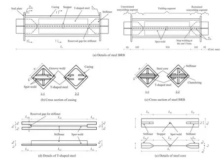
Fig.1 Specimen setup

However,assessing the hysteretic behavior and ductility of BRB components through real experiments is expensive,especially considering the heavy dependence on experimental-based techniques (Jouneghani and Haghollahi,2020;Zhaoet al.,2022).Moreover,testing of BRB components may not be feasible due to the size and strength of the structural members.Considering these issues,reliable simulation and prediction techniques for BRBs are highly attractive and allow for improved practicality in modeling the effects of diverse material properties and loading conditions at the component level.

Recently,several numerical studies have been conducted to enhance and facilitate the use of BRBs in high-risk seismic buildings (e.g.,Fahnestocket al.,2003;López-Almansaet al.,2012;Hoveidae and Rafezy,2015).For example,Hoveidae and Rafezy (2015) conducted a numerical investigation of the seismic behavior of short core BRBs to demonstrate their feasibility.Budaházy and Dunai (2015) carried out a numerical analysis of concrete-filled BRBs,in which a novel Chaboche-based constitutive model was developed in the ANSYS finite element environment to model cyclic steel plasticity with combined hardening.It was concluded that the developed FE model could accurately replicate the features of BRBs observed during the tests.AlHamaydehet al.(2016) conducted a numerical study on BRBs to investigate the most influential BRB design parameters through the finite element method.It was concluded that the necking of the core was potentially the most serious factor in influencing the ductility of BRBs.Shiet al.(2018) carried out complementary FE simulations to determine the energy dissipation mechanism of all-steel assembled low-yield-point BRBs,in which a simple bilinear kinematic hardening model was utilized to capture the response of the core plate.

The aforementioned BRB FE models were developed in Abaqus or ANSYS,and the steel material was modeled with different constitutive models (from simple bilinear to complex combined hardening).In a prior paper by Jianget al.(2020),the numerical analysis was treated as a complementary method to contrast with the experimental results.Given that,it was necessary to provide comprehensive insight into the most influential BRB design parameters through finite element analysis and propose some recommendations for further applications.

2 Research objectives

The simulation of complex physical events has long been a focus of the academic community.Simulation models reduce the necessity of exhaustive experimentation and extend experimentally observed phenomenon to cases that may be difficult to test.Thus,through the application of theoretical and analytical models,routine design and construction need not rely on the testing of a replicate structure.Furthermore,the testing of a replicate structure would be impractical,and in many cases,an impossible feat.

In this regard,a finite element analysis of the allsteel buckling-restrained brace proposed by Jianget al.(2020) is presented in this paper.

This study first emphasizes the constitutive models applied to the core plate.Compared with the simple bilinear hardening model utilized in Jianget al.(2020),a more advanced constitutive model (Chaboche model(Chabocheet al.,1979)) is introduced to accurately capture the global and local responses of the core plate under cyclic loadings. To implement this constitutive model,the corresponding calibration process of the model parameters is also illustrated in detail.

Second,a detailed description of structural modeling techniques in the context of the BRB components proposed by Jianget al.(2020) is presented.To validate the accuracy of the FE model,comparisons with the experimental results depicted in the prior study are also carried out.Meanwhile,the simulated results from the same FE model with different constitutive models (from simple bilinear to complex combined hardening) are also conducted to demonstrate the superiority of the advanced material model.Furthermore,the advanced constitutive model is selected as a benchmark model to optimize the most influential BRB design parameters for further application.Among the design parameters of this novel BRB to be considered herein are the initial imperfections of the core,the friction coefficient and clearance between the core and the T-shaped plate,the cross-section widththickness ratio (or the compactness ratio) of the core,and the thickness of the T-shaped plate and angle steel.In addition,the BRB ductility evaluation indicators considered are compression strength adjustment factor and equivalent viscous damping coefficient.

3 Steel constitutive model

It is well known that metal plasticity at room temperature is recognized as rate-independent,in which hydraulic pressure has little impact on the metal plasticity.Thus,for metal plasticity,the Mises yield function and the associated flow rules are universally accepted and are applied herein.In this section,the primary concern is the hardening rule.Generally,there are two basic hardening rules to describe the changes of the yield surface in the principal stress space.The first hardening rule is isotropic hardening,taking into consideration the stretch of the yield surfaces.Figure 2 presents the most commonly used isotropic hardening model.The other rule is kinematic hardening,which allows for the movement of the yield surface in the primary stress space.Figure 3 demonstrates the simplest kinematic hardening model.

Fig.2 Representation of linear isotropic hardening model

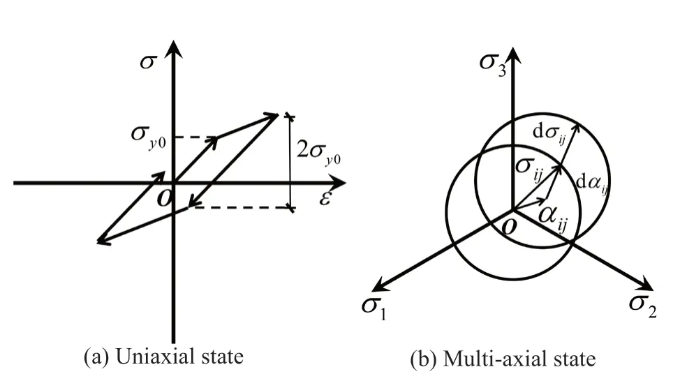
Fig.3 Representation of linear kinematic hardening model

Isotropic hardening is introduced through a scalarRto describe the stretch of the elastic domain.The value ofRcan be positive (cyclic hardening) or negative (cyclic softening).The scalarRis usually defined as the function of equivalent plastic strain as:

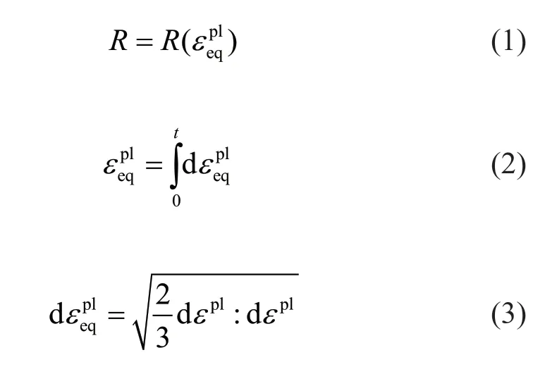
whereis the equivalent plastic strain,is the incremental equivalent plastic strain,andis the tensor of the incremental plastic strain,which is determined from the associated flow rules based on the normality hypothesis.In addition,‘:’ denotes the contract product of two second-order tensors.The isotropic part of the hardening can be expressed as the function of equivalent plastic strain in the exponential form:

whereQis the asymptotic value of the scalarRin the infinite strain or the stabilized hysteresis loops,andbdetermines the rate of stabilizing.This nonlinear hardening rule can describe the behavior of cyclic loaded structural steel but cannot model the decrease of the initial yield surface,which will be illustrated in the following sections.

Most of the available kinematic hardening rules are developed based on the simple bilinear hardening law proposed by Prageret al.(1949).In the Prager model,the yield surface movement in stress space is defined by a particular stress tensor,termed as backstressα,which can be expressed as follows:

whereCis a material parameter determined through uniaxial tensile tests.The Prager model with Mises yield criterion can be expressed as follows:

wherefis yield function,sandαare the deviatoric stress of Cauchy stress and backstress,respectively,andσy0is the initial yield stress.It has been pointed out that the linear kinematic hardening law is too rough to predict the kinematic hardening components of the structural steel under cyclic loading and is only reasonable within a strain range of 5%.Thus,a series of material models have been developed from the simple bilinear hardening model.Armstrong and Frederik (1966) modified the Prager model by introducing a relaxing term called dynamic recovery into the backstress.The relaxing term(recall term) was introduced to describe the evanescent strain memory effect (evanescent along the plastic strain path),and can be written as follows:

whereCandγare material parameters,and 2/3 is chosen to make the expression a unity form under uniaxial tensile loading.In addition,Cdenotes the initial hardening modulus,andγis the nonlinear recover parameter,which introduces a fading memory effect of the strain path.Using monotonic tensile loading as an example,Eq.(8) can be written as follows:

Integrating Eq.(9) under isothermal conditions withα(0)=0 and(0)=0 gives

Generally,the A-F model is more accurate than the simple bilinear hardening model (Prager model).However,a single nonlinear kinematic hardening model cannot adequately replicate the cyclic behavior of structural steel,since it has been demonstrated that the kinematic hardening components have different evolution rates at different strain ranges.Thus,Chabocheet al.(1983) discovered that the material nonlinear hardening behavior at different strain ranges could be better simulated by superimposing a combination of different A-F formulas.As shown in Fig.4,the Chaboche model with several backstresses is written as follows:

Fig.4 One-dimensional representation of the Chaboche model with isotropic hardening

whereiαis theith backstress,iCandiγare model parameters of theith backstress,and n is the total number of backstresses.The original Chaboche model is simply a pure kinematic hardening model.To consider the stretch of the yield surface,the aforementioned isotropic hardening law is introduced.

4 Calibration of the model parameters

Since the advanced constitutive models have been proposed,it is necessary to calibrate the relevant material parameters to apply these models.This section will illustrate the model parameter calibration and the relevant coupon tests in detail.

4.1 Tension specimens

Steel coupons for uniaxial tensile testing are machined using the same steel plates applied to the BRBs proposed by Jianget al.(2020).In the prior study,Q235B steel is utilized for the core,while Q345 steel is used for the remaining components of the all-steel BRB.Thus,six tension specimens (each steel material with three specimens) are manufactured based on the Chinese tensile test codes.The configurations and dimensions of the specimens are shown in Fig.5 and listed in Table 1,respectively.The thickness of the specimens is 10 mm,taking into consideration the thickness of the core plate as well as the capacity of the loading machine.According to the Chinese codes,a plastic length is designed to ensure that the gradients of the stress and strain are moderate.Meanwhile,the specimen′s transition parts are configured in an arc-shaped fashion to preclude the premature instability.Special care is taken in the machining process to reduce changes in the physical surface and material properties of the specimens.Furthermore,all the tension specimens are extracted in the rolling direction of the steel plate,considering the large dispersion of material properties perpendicular to the rolling direction.

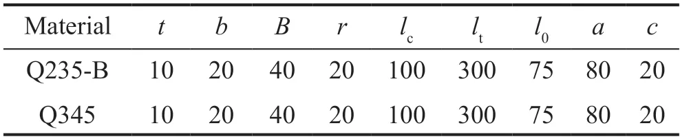
Table 1 Dimensions of coupon test specimen (unit: mm)

Fig.5 Setup of the coupon test specimen

4.2 Test setup

The uniaxial monotonic tension tests are conducted in the Key Laboratory of Earthquake Engineering and Engineering Vibration of the China Earthquake Administration,in Harbin.The specimens are screwed into the grips of the AG-250KNI universal testing machine,which provides the capability of testing under load or displacement control.The load readout is monitored by the calibrated load cell built in the machine,which is synced with a digital high-speed data logger.High-elongation single element strain gauges are utilized to measure the longitudinal strains in the coupons′ gauge zone.The strain gauges are glued on opposite sides of the tension specimens to eliminate bending effects (shown in Fig.6).In addition,another two strain gauges are glued perpendicular to the longitudinal direction of the specimens to determine the Poisson′s ratio of the steel.The uniaxial tensile tests are conducted at a quasi-static loading rate of 0.06 mm/min up to yield and increase to 0.24 mm/min after yield.Meanwhile,the load and strain data are stored through the data logger at time intervals of 0.5 s.The data of extension reading from the machine is employed to monitor the displacement response of the test specimens and not for numerical analysis because these data lack accuracy.The setup of the test system is shown in Fig.6,and the corresponding nominal stressstrain curve is shown in Fig.7.

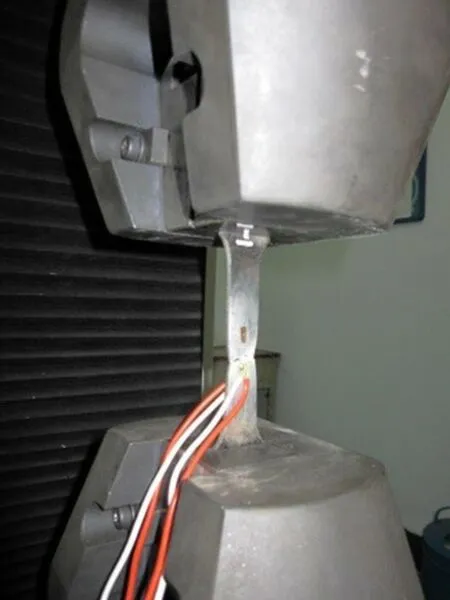
Fig.6 Test set-up

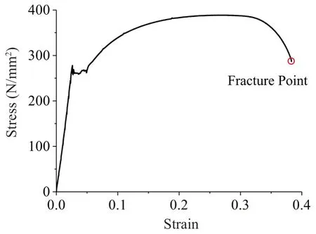
Fig.7 Stress-strain curve of Q235B

4.3 Determination of material parameters

4.3.1 Initial yield stressσy0,Young′s modulusEand Poisson′s ratioν

Young′s modulusEis defined as the gradient of the initial linear part of the stress-strain curve.In addition,Poisson′s ratioνis defined as the negative transverse strain divided by the axial strain in the direction of the stretching force,in which the strains can be obtained from the strain gauges glued in the two orthogonal directions (see in Fig.6).The initial yield stressσy0can be approximated as the stress at 0.2% off-set strain.

4.3.2 Isotropic hardening parameters,Qandb

Equation (13) indicates that as the equivalent plastic strain increases, exponentially approaches to the asymptotic valueQ.This assumes that the material hardening observed in the monotonic tensile test is entirely due to the isotropic hardening.While plottingRagainst the equivalent plastic strain,the asymptotic value ofRis defined asQ.Furthermore,using nonlinear least squares regression,Eq.(13) can be fitted to the experimental model from the yield strain until the necking strain,and hencebcan be identified.

In this section,the stress and strain used for parameter calibration are the true stress and strain,considering the reduction of the cross-sectional area.The true stress can be written as

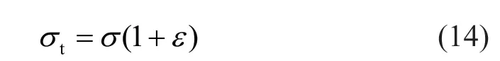
whereσandεare the engineering stress and strain,respectively.

In addition,the true strain is given as,

wheretεis the true strain.In the case of the uniaxial tensile loading,the equivalent plastic strain is the same as the accumulated plastic strain,and can be expressed as follows:

The above definitions are valid only until necking initiation.After necking initiation,the stress state in the necking zone becomes triaxial,and the study of material behavior after necking initiation is out of the scope of this research.Detailed investigations can be found in Jia and Kuwamura (2015).

4.3.3 Kinematic hardening parameter for Prager model,C

The calibration of the kinematic hardening modulusCdepends on the strain range of concern.Generally,the linear kinematic hardening modulus,C,is determined from the relation.

In this study,the peak true stress and the corresponding equivalent plastic strain are utilized to determine the material parameter.

4.3.4 Kinematic hardening parameters for Chaboche model,Ciandiγ

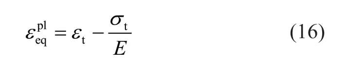
In this section,the hysteretic responses of the first three stabilized hysteresis loops of an all-steel BRB are utilized to identify the model constants.For one stabilized hysteresis loop,a series of the true stressstrain data pairs (σt,i,εt,i)can be calculated using Eqs.(14)-(16).Moreover,each true stress-strain data pair must be specifically reformulated intowith the strain axis shifted to,so that

whereσs= (σt,1+σt,n)/2is the stabilized size of the yield surface.

Integration of the back-stress evolution laws over this stabilized strain cycle,with an exact match for the first data pair(σt,1,0),provides the expressions

whereαi,1denotes theith back-stress at the first data point (the initial value of the back-stress),andNis the total number of the back-stresses at each data pair.The above equations enable calibration of the parametersCiandγi.

Obviously,the calibration results tend to be more accurate with a larger value ofN.Considering the balance between the computational expense and accuracy,the number of back-stressesNis taken as an appropriate value of 4 herein.The first kinematic hardening componentα1,predominantly signifies the first loop section by initiating a very large slope followed by quick stabilization.The fourth kinematic hardening componentα4with a small value ofγ4signifies the fourth loop section,which is nearly linear along with a slight slope.The transition part of the hysteresis curve is partitioned into two sections,which are represented principally by the second and third kinematic hardening components.

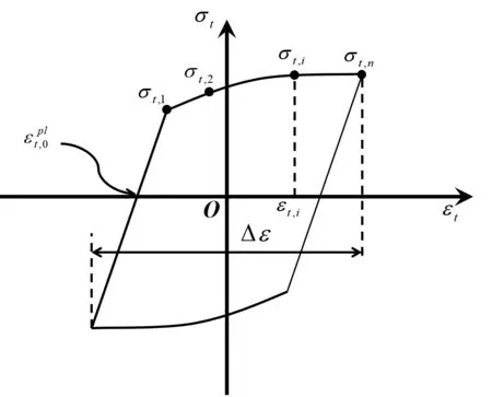
Fig.8 Stress-strain data for a stabilized cycle

Given the above elaboration,the kinematic hardening material parameters can be determined through the data pairsof the stress-strain curves obtained at different strain ranges,which can be entered directly in Abaqus.The calibrated values corresponding to each strain range are reported in the data file,together with an averaged set of parameters,if model definition data are requested.

5 Finite element modeling of the steel BRB

To characterize the hysteretic responses over the course of the loading history,finite element models are created for the BRB components.The required variables,such as the reaction force and loading displacement,can then be extracted and input into the characteristic equations of the ductility evaluation indicators to determine the hysteretic responses as predicted by the calibrated model.The components of the all-steel BRB are modeled using the general-purpose finite element analysis program ABAQUS,which incorporated material strain-hardening/ softening and large geometric deformation.To simplify the weld joint,rigid links are introduced to model the connectors between the stiffener and the core.Given that the T-shaped steel is tightly fastened to the casing,tie constraints are utilized to model this connection.Furthermore,there is no doubt that the core would come into contact with the T-shaped steel and casing while under compression.Considering this highly nonlinear behavior,the contact properties are established between the core and the restraint members to model the sliding behavior,incorporating both normal and tangential behaviors of the contact interface.The frictional coefficient is introduced to model the tangential behavior on the contact interface.The penalty contact model is utilized to model normal behavior.In this contact model,the core′s surface is considered “penetrating master,” while the T-shaped one is “penetrated slave,” and the penetration is described with a penalty formulation by interposing a highly stiffspring between both surfaces.In addition,the penalty contact model is also applied to simulate the interactions between the stopper and T-shaped steel.Hence,the stopper mechanism can also be introduced in the numerical analysis as expected.Moreover,the damping factor for contact control is set to be 1×10-4to achieve a better convergence during simulations.

To accurately reflect experimental conditions,the loading displacements are applied to a control node at the center of the rectangle near the end of the core.As shown in Fig.9,the surface of the rectangle at the end of the core is “slaved” to the master node such that,for all degrees of freedom,any displacement applied to the master node would also be applied to the overall rectangular surface at the end of the core.The numerical analyses are run in displacement control with the loading protocol described in Fig.10,which is consistent with the loading history adopted in the quasi-static experiments.The amplitude function is utilized to recreate the cyclic loading protocol.As mentioned above,the loading protocol is applied to the master node,which “forces”the same displacement history to the slaved surface due to the rigid coupling constraint.Finally,a fixed boundary condition is applied to the other end of the core to model the connection between the BRB component and the bracing member.

Fig.9 Coupling restraint

Fig.10 Graphical expression of loading protocol

The finite element meshing criteria for the BRB component should be chosen carefully to achieve the following objectives: to allow for solution convergence,to closely follow the geometry of the component,and to minimize the analysis time.Due to the BRB components′complex geometry,C3D8R with reduced integration and linear shape function elements are chosen to mesh the assembly,taking into consideration minimizing the analysis time for the large FE models.The general mesh size is chosen so that there are at least four elements through the thickness of the steel core,which is intended to preclude the undesired hourglass effect typically observed on reduced integration elements.To minimize the computational expense,the mesh size of the T-shaped steel and casing are relatively coarse compared with that of the core.Figure 11 depicts the typical meshes for various cross-sections,comprising 18,228 elements.According to the figure,the mesh is more refined at the center of the core,where severe plastic deformations are expected.

The simple bilinear hardening model and nonlinear combined isotropic and kinematic hardening model(Chaboche model) are chosen to describe the behavior of the finite element models.Both constitutive models are applied to the core to investigate the superiority of the advanced material model.In addition,the simple bilinear hardening model is assigned to the T-shaped steel and casing,considering the computational expense.Based on the suggestions illustrated in Section 4,the appropriate material model parameters are determined for applying the Prager model and Chaboche model to metal plasticity.These material hardening parameters are provided as listed in Table 2.

Moreover,the BRB finite element models are executed with nonlinear geometric effects to consider any second-order geometric effects that may be captured throughout the loading protocol.The direct solver is also implemented with full Newton integration,linear extrapolation of the previous state at the start of each increment and loading ramped linearly over the step.The BRB component model analysis duration is approximately two hours using four parallel processing 2.5 GHz cores with 8 GB of RAM.

Since the initial defects responsible for the fracture are triggered by the fabrication and welding flaws,it is important to accurately replicate these events in the BRB simulations.To achieve this,global imperfection is introduced to the BRB model by scaling the eigenvectors from the elastic buckling analysis.The elastic buckling analysis is performed using Abaqus to determine the buckling shapes of the core.The global buckling analysis involves applying a compressive load at the end of the core,where the loading displacement is applied.Figure 12 demonstrates the first three buckling modes obtained from the elastic buckling analyses for the core.The global imperfections are introduced by scaling the first global buckling mode shape,such that the peak deflection at the center is equal to 1/1000 of the BRB length,which is the maximum sweep of compression members assumed by AISC (2005).Thus,the elastic global buckling eigenvector is scaled such that the maximum out-of-plane imperfection is taken as 0.655 mm in the FE model.

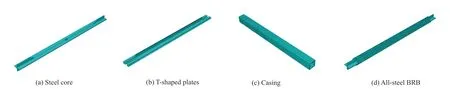
Fig.11 Finite elements meshing of the BRB

6 Hysteretic performance assessments

Numerous research studies have been conducted to investigate different types of BRBs in recent decades.Hence,some generally accepted criteria have been proposed to evaluate the overall ductility of BRBs.The subsequent section will review several assessment indexes typically used in the literature.

(1) Compression strength adjustment factor,β:

Due to the confining effect of the T-shaped steel and casing,the maximum compressive strength of BRB is usually higher than the maximum tensile strength.This small unbalance must be considered from a capacity design point of view.If not correctly designed,this component property can create a large imbalance force on the beam (in the chevron-type configurations of BRB frames).Hence,the compression strength adjustment factorβis introduced to characterize this over-compression property:

whereCmaxandTmaxdenote the maximum compressive and tensile strength of the specimens,respectively.

(2) Equivalent viscous damping,he:

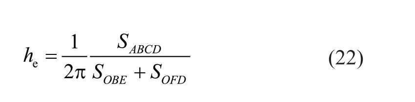
The energy dissipation capacity of BRB is usually determined by calculating the area within each forcedeformation cycle.To normalize the energy dissipation,the equivalent viscous dampingheis introduced,which is defined by the ratio of the dissipated energy (the area ofABCD) to the absorbed energy (the area ofOBEandOFD) of the equivalent elastic component that undergoes the same displacement (see in Fig.13).Reviewing the literature about BRBs,the load-deflection curves of all-steel BRBs are usually idealized in a bilinear form.Thus,the absorbed energy (i.e.,the maximum elastic strain energy for the cycle) can be calculated as half the product of the maximum force and the corresponding maximum deformation for the cycle.The equivalent viscous damping,hefor a given deformation cycle is calculated by the following expression:

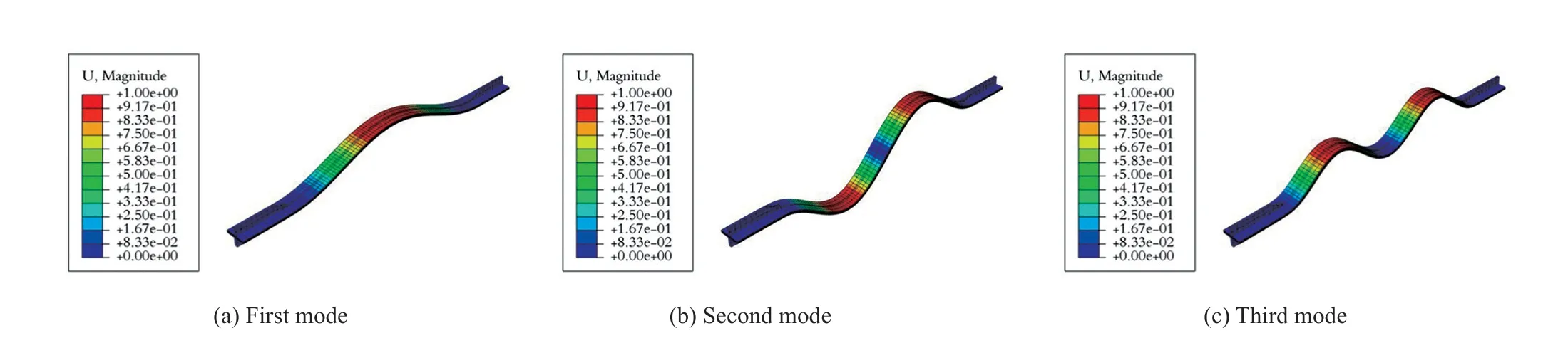
Fig.12 First three buckling modes of the core

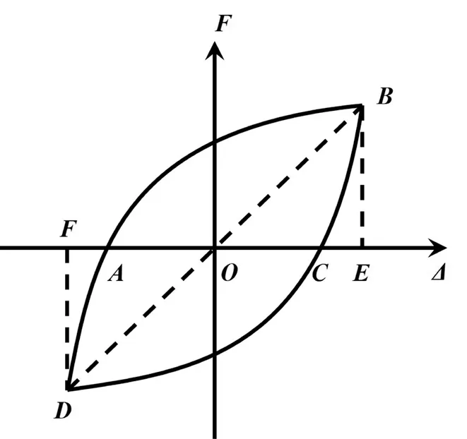
Fig.13 Definition of he

7 Comparisons between experimental and simulated results

To validate the accuracy of the FE model,the comparisons between the experimental and simulated results are conducted using the abovementioned assessment methods.In this section,all the comparisons are made based on the Q-series specimens proposed by Jianget al.(2020),whose dimensions are listed in Table 3.Figure 14 shows the Mises stress contours of the Q-4 FE model at the maximum compressive.As depicted in Fig.14,the core is the main component tosustain large compressive plastic deformations,and the contact region between the core and casing exhibited a higher stress level,which reveals that the thrust forces generated by the core are responsible for the design of the casing.In addition,the plastic zones (red in Fig.14(a))of the core are not evenly distributed in the contact region,and the two ends of the core and the casing in the contact regions almost remain elastic as expected.

Fig.14 Von-Mises stress contours of the BRB under maximum compression (unit: N/m2)

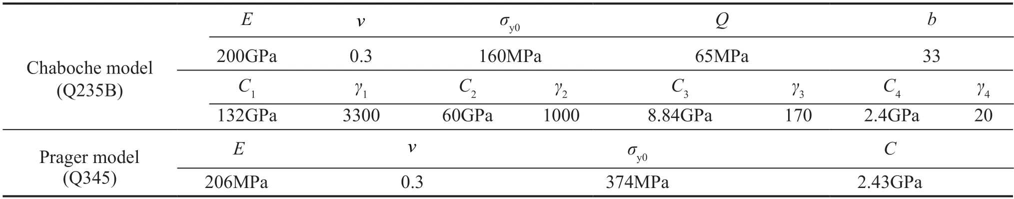
Table 2 Calibrated model parameters of plasticity model

Figure 15 demonstrates the local buckling modes of the steel core under incremental compression inelastic excursions.As illustrated in this figure,the buckling mode progressively evolves from the simple half-sine shape (corresponding to the initial imperfection that was specified in Fig.12) to higher modes.In the initial phases,the contact points between the steel core and the casing are concentrated at the core end and core mid-span.With the development of inelastic compression displacements,the number of contact points then gradually increases with more pronounced curvature,and the contact points are also closely spaced at the core ends.

In Table 4,it can be observed that the maximum tensile and compressive strengths obtained from the simulated results are almost identical to the experimental results.Due to the definition of the compression strengthadjustment factor,there is no doubt that the simulated results concerningβshould be kept consistent with the experimental results,which range from 1.08-1.12,satisfying the upper limit of 1.3 specified in the AISC Seismic Provisions.As for the constitutive models applied to the core,the simulated results utilizing the nonlinear combined isotropic and kinematic hardening model are closer to the experimental results,compared with those using simple bilinear model.

Table 3 Specimen sizes (unit: mm)

Figure 16 presents a comparison of the hysteretic curves between the experiments and FE simulations.The simple bilinear model simplifies the skeleton curve into two linear parts and cannot accurately capture the transient Bauschinger behavior.This is illustrated in Fig.16(a),where the hysteretic curves resulting from the simple bilinear model are not particularly consistent with the experimental results during the reversal loading phase.Figure 16(b) compares the experimental response of Specimen Q-4 with the numerical simulation obtained from the nonlinear combined model.It is seen that the numerical responses with nonlinear combined models fit well for the fully developed cycles controlled by kinematic hardening.During the reversal loading phase,the hysteretic curves almost coincide with the experimental ones.However,this model,with a constant relationship between the isotropic and kinematic hardening components,usually under-estimates the material hardening,especially in the initial cycles,where the higher isotropic hardening component is dominant.Thus,the BRB yielding strengths predicted by the nonlinear combined model is lower than the experimental results.

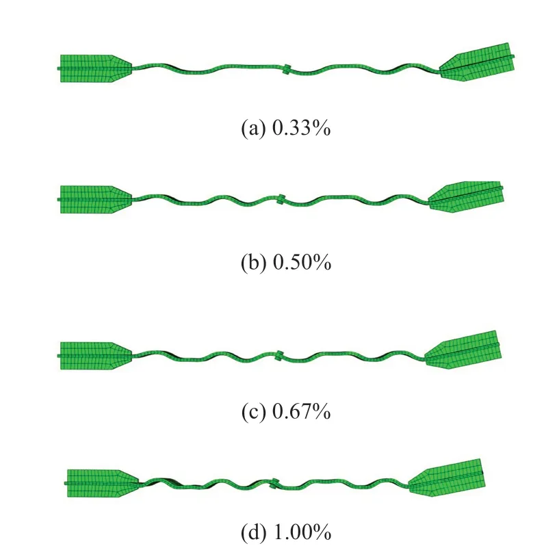
Fig.15 Evolution of the buckling mode of steel core at maximum compression displacement at Δ=0.33%Lt,0.67%Lt,1.00%Lt (×10),respectively

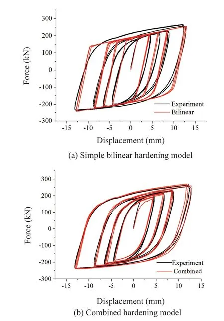
Fig.16 Hysteretic curves comparisons between experiments and FE simulations

Figure 17 presents the backbone curve comparisons between the experiments and FE simulations.It can be observed that the FE simulations using the bilinear model are in good agreement with the experimental results,which indicates that the bilinear assumption is reasonable.As mentioned previously,the numerical responses with the nonlinear combined models are inconsistent with the experiments during the initial cycles.The reason for this significant inaccuracy lies in the fact that the isotropic part of the hardening cannot model the yield plateau and the decrease of the initial yield surface.As the plastic strains accumulate,this inconsistency gradually disappears,and the strengths predicted by the advanced constitutive model are closer to the experimental results than those determined by a simple bilinear model.A similar trend can also be found in Fig.18,where the dissipated energies are compared between the experimental and simulated results.Figure 19 presents the equivalent viscous damping comparisons between the experiments and FE simulations.The results predicted by the nonlinear combined models are in good agreement with the experimental results except for the first cycle.However,the FE simulations using the bilinear model are consistent with the experimental results during the initial cycles.After several cycles,the results predicted by the simple bilinear model gradually deviate from the experiments.

Fig.18 Energy dissipation comparisons between experiments and FE simulations

Given the above elaboration,the results predicted by the simple bilinear model and the nonlinear combined models are almost consistent with the experimental results,which directly validate the accuracy and effectivity of the FE model.Compared with the simple bilinear model,the numerical responses with the nonlinear combined model fit better with the experimental results except for the initial cycles.In addition,the nonlinear combined model can model the transient Bauschinger effect so that the hysteresis loops predicted by this model are closer to the experimental curves during the reversal loading.Considering the accuracy of the global and local responses mentioned above,it is reasonable to select a nonlinear combined model for the optimal design process.

8 Optimal design process based on BRB FE model

The aforementioned FE model makes it possible to analyze the typical characteristics of BRB components.Considering that different configurations would result in different hysteretic behavior,it is necessary to make some general requirements to ensure the performance of the device.As mentioned previously,there are several parameters to characterize this device,including(i) the compression strength adjustment factor (β),which represents the over-compression;(ii) the strain hardening adjustment factor (ω),which describes the work hardening under tension;(iii) the cumulative plastic ductility (CPD),which defines the cumulative plastic deformation;and (iv) the equivalent viscous damping coefficient (he),which demonstrates the change of energy dissipation during cyclic loading.It is obvious that the tensile excursions of the hysteretic loops hardly differ from the material constitutive model,regardless of the configurations of BRBs.In addition,the failure criterion is not involved in the material constitutive model;therefore,the cumulative plastic ductility is determined by the loading protocol,regardless of the configurations of BRBs.Thus,the parametric investigations focus on the compression adjustment factors and the equivalent viscous damping coefficients of BRBs.Furthermore,among the design parameters influencing the cyclic performance of the device to beconsidered in this study are the initial imperfections of the core,the friction coefficient and clearance between the core and the T-shaped plate,the cross-section widththickness ratio (or the compactness ratio) of the core and the thickness of the T-shaped plate and angle steel.These parameters are fundamentally different depending on the manufacturer;therefore,it is necessary to give general recommendations for these design details through the finite element method.Meanwhile,the FE model of the Q-4 specimen is selected as the benchmark model for the parametric investigations,and the relevant design parameters to be considered are listed in Table 5.

Table 4 Hysteretic responses comparisons between the experiments and FE simulations

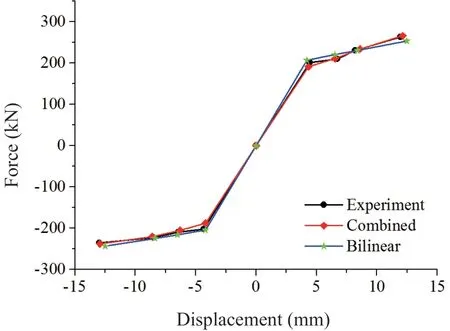
Fig.17 Backbone curves comparisons between experiments and FE simulations

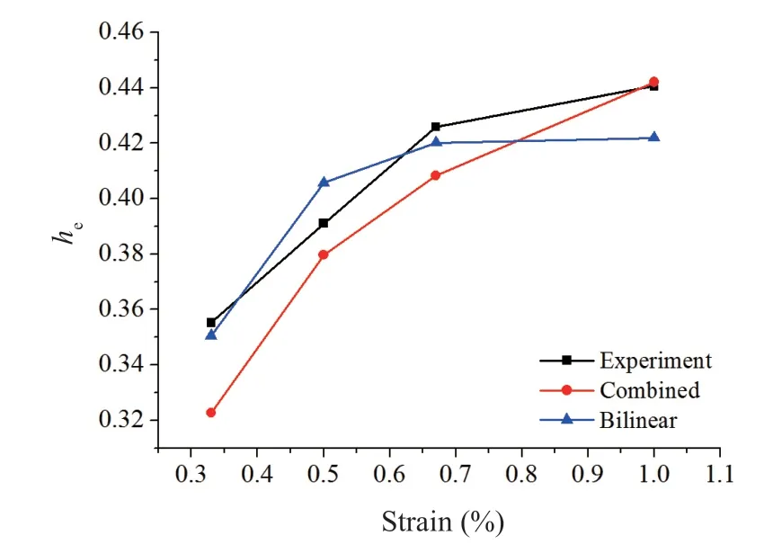
Fig.19 Equivalent viscous damping comparisons between experiments and FE simulations

8.1 Parametric investigations on the initial imperfections

The previous sections have mentioned that equivalent geometrical imperfection can be introduced through scaling the eigenvectors from the elastic buckling analysis in Abaqus,and the elastic buckling analysis is performed to determine the two perpendicular axis buckling shapes of the core.In the previous sections,the imperfection amplitude is set to 1/1000 of the BRB length,which is the maximum sweep of compression members assumed by AISC (2005).In this section,a detailed parametric study on the initial imperfections is conducted through varying the imperfection amplitudes.The maximum imperfection amplitude is set to the gap between the core and T-shaped steel,which is large enough to develop the geometrically nonlinear phenomenon but does not cause initial convergence problems due to contact.The minimum imperfection amplitude is set to be zero,which indicates the core is in a perfect state.

As listed in Table 6,it is obvious that the imperfection amplitude has little impact on the compression strength adjustment factor.Nevertheless,there is a slight trend thatβdeclines with the rise of the imperfection amplitude.Figure 20 shows the hysteretic curve,the dissipated energy,and the equivalent viscous damping comparisons among different imperfection amplitudes.It can be concluded that the imperfection amplitude has little influence on the hysteretic behavior of this all-steel BRB.Despite this,Fig.20(c) reveals that 1 mm is a better choice for the imperfection amplitude,taking into account the equivalent viscous damping consideration.

Table 5 Design parameters for the all-steel BRB

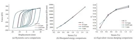
Fig.20 Hysteretic behavior comparisons among different initial imperfections

8.2 Parametric investigations on the friction coefficient

The friction coefficient between the core and the T-shaped plate is an important design parameter.During compressive excursions,the core has contact with the T-shaped steel;therefore,the transfer of shear force occurs between the restrained segment and casing.The transfer of shear force can directly increase the axial compressive demands on the core,accelerating the over-compression of BRBs.Thus,it is necessary to determine the influences of the friction coefficient on the performance of the device and give specialrecommendations for this design parameter.

As listed in Table 7,the friction coefficient greatly impacts the compression strength adjustment factor.With the increase of the friction coefficient,the compression strength adjustment factorβremains upward.It is the friction coefficient that characterizes the over-compression of this all-steel BRB.Figure 21 demonstrates the hysteretic curve,the dissipated energy,and the equivalent viscous damping comparisons among different friction coefficient,respectively.It is interesting to note that the compressive strength will drop abruptly when the friction coefficient is zero.Meanwhile,by augmenting the friction coefficient,the all-steel BRB dissipates more energy under the same axial strain.However,the equivalent viscous damping presents an opposite trend.This result can be attributed to the increasing compressive strength and constant tensile strength under the incremental friction coefficient.Considering the balance between the dissipated energy and equivalent viscous damping,0.1 is a better choice for the friction coefficient.

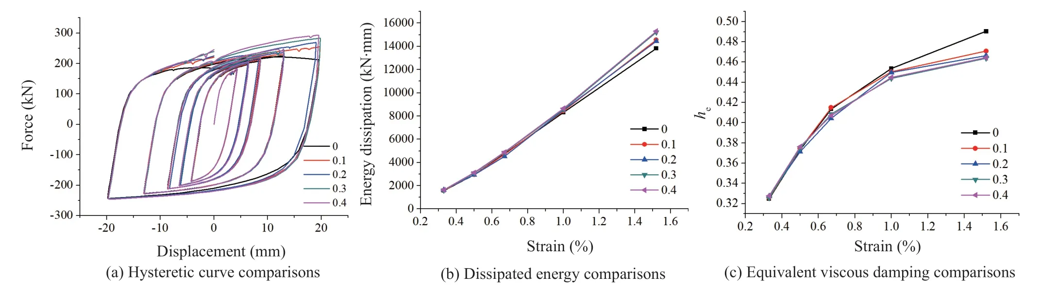
Fig.21 Hysteretic behavior comparisons among different friction coefficients

8.3 Parametric investigations on the air gap

The air gap or the clearance between the core and the T-shaped plate is vital to the performance of the core.Maet al.(2010) found that moderate air gaps should be appropriate.If the air gaps are restrained in a reasonable range,the amplitude of buckling will be rather limited,and consequently,the contact forces and frictions can also be moderated.However,relatively small air gaps may cause the core to jam due to the transverse contraction of the core in compression.Thus,several discrete,constant air gap sizes are investigated in this section to give special recommendations for this design parameter.

As listed in Table 8,the compression strength adjustment factorβremains invariable under different air gaps.Figure 22 demonstrates the hysteretic curve,the dissipated energy,and the equivalent viscous damping comparisons among different air gaps.The hysteretic behavior becomes unstable when the air gap is set to 2 mm.The increasing local buckling amplitude may be responsible for this undesirable result.Consideringthe balance between the hysteretic performance and fabricating accuracy,1 mm is a better choice for the air gap between the core and the T-shaped plate.

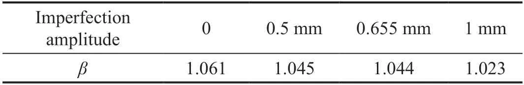
Table 6 Variation of the compression strength adjustment factor

Table 7 Variation of the compression strength adjustment factor

8.4 Parametric investigations on the compactness ratio of the core

The cross-section width-thickness ratio (or the compactness ratio) of the core is responsible for the local buckling of the BRB component.Jianget al.(2020)proposed that the compactness ratio of the core should be limited to a reasonable scope;consequently,the thrust force generated by the core can also be moderated.In addition,the compactness ratio of the inner core should be appropriate to ensure the dissipation performance of the BRB component.Thus,several discrete compactness ratios of the core are investigated in this section,while keeping the same casing to ensure that the quantitative results are confidential.

Table 9 reveals the relationship between the compression strength adjustment factorβand the compactness ratio of the core.It can be concluded that the compactness ratio should not be larger than 20;otherwise,the compression strength adjustment factor would exceed the upper limit of 1.3 specified in the AISC Seismic Provisions.In addition,there is no evident difference whenever the compactness ratio is set to 8 or 10.Figure 23 demonstrates the hysteretic curve,the dissipated energy,and the equivalent viscous damping comparisons among different compactness ratios,respectively.When the compactness ratio is set to 20,the hysteretic curve shows obvious oscillation,especially during larger compressive strains.Moreover,the equivalent viscous damping,in this case,is inferior to those in the other two cases.Considering the hysteretic performance,8 or 10 seems to be a better choice for the core′s compactness ratio.

Fig.22 Hysteretic behavior comparisons among different air gaps

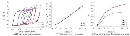
Fig.23 Hysteretic behavior comparisons among different compactness ratios

8.5 Parametric investigations on the thickness of the casing

The thickness of the casing of this type of BRBs is also an important design parameter.Jianget al.(2020)found that the thickness of the casing is essential in the global behavior of the steel BRB.There is no doubt that the thicker the casing,the higher the flexural strength of the BRB component.However,manufacturing costs must be considered from an economical design point of view.Hence,several discrete thicknesses of the casing are investigated to seek an optimal value.Four different thicknesses of the casing are investigated (2,3,4,6 mm)with the same core.The results are shown in Fig.24 andTable 10.Although the cross-sectional areas of the cores are equal,significant global buckling can be observed in the BRB with a thinner casing,caused by the larger outof-plane displacement of the yielding zone.As shown in Fig.24,when the thickness of the casing is smaller than 3 mm,the steel BRB exhibits obvious global buckling instability.Thus,4 mm is an optimal value for the casing of this steel BRB.

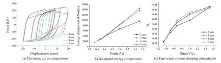
Fig.24 Hysteretic behavior comparisons among different thicknesses of the casing

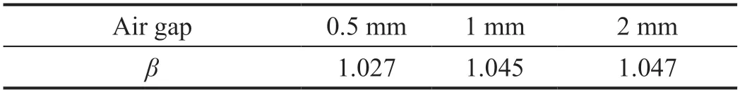
Table 8 Variation of the compression strength adjustment factor

Table 9 Variation of the compression strength adjustment factor

Table 10 Variation of the compression strength adjustment factor

9 Conclusions

In this study,a detailed numerical analysis of the allsteel BRBs,proposed by Jianget al.(2020),has been conducted.As Part II of the entire research project,this paper aims to provide general recommendations for the design details of this novel all-steel BRB through the finite element method.To this end,two different steel constitutive models are introduced to precisely capture the hysteretic behavior of the core under cyclic loading.Meanwhile,a particular calibration process of the model parameters is proposed to apply the two models.

In order to characterize the hysteretic responses,finite element models are created for the BRB components.Meanwhile,the finite element procedures are elaborated in detail for the following optimal design process.To validate the accuracy of this finite element model,comparisons with the experimental results,depicted in the prior study,are first carried out.Then,comparisons between different steel constitutive models are performed to demonstrate the superiority of the nonlinear combined hardening model.According to the results,the simulated results are in good agreement with the experimental results in predicting the global behavior of the BRB component.Moreover,the finite element model with a nonlinear combined hardening model can predict more accurate results than that with a linear hardening model.Nonetheless,the Chaboche model with a constant relationship between the isotropic and kinematic hardening components usually underestimates the material hardening,especially in the initial cycles.Thus,the yielding strength predicted by this model is somewhat lower than the experimental results.This shortcoming can be improved by introducing an additional parameter to dynamically adjust the proportion of the isotropic hardening component,which is out of the scope of this study.Based on the comparison results,the finite element method with a nonlinear combined hardening model is utilized for the deeper parametric analysis.

The optimal design process is conducted to make some general recommendations for the device.According to the parametric analysis,the performance of this novel steel BRB is not sensitive to the initial imperfections of the core.In addition,it is the friction coefficient between the core and the T-shaped plate that characterizes the over-compression of the BRBs,and 0.1 is recommended as the friction coefficient.As for the air gap between the core and the T-shaped plate,1 mm seems to be a better choice considering the hysteretic performance and fabricating accuracy.Furthermore,it is observed that 8 or 10 is a better choice for the compactness ratio of the core.The results also reveal that 4 mm is an optimal value for the casing of this novel steel BRB,which considers the manufacturing cost of the BRB component.Through the optimal design process,this BRB with detailed configurations can provide excellent hysteretic behavior and seismic performance.