Stability conditions of explicit integration algorithms when using 3D viscoelastic artificial boundaries

Bao Xin ,Liu Jingbo ,Li Shutao ,Wang Fei and Lu Xihuan

1.Department of Civil Engineering,Tsinghua University,Beijing 100084,China

2.Institute of Defence Engineering,AMS,PLA,Beijing 100036,China

3.College of Defense Engineering,Army Engineering University of PLA,Nanjing 210007,China

Abstract: Viscoelastic artificial boundaries are widely adopted in numerical simulations of wave propagation problems.When explicit time-domain integration algorithms are used,the stability condition of the boundary domain is stricter than that of the internal region due to the influence of the damping and stiffness of an viscoelastic artificial boundary.The lack of a clear and practical stability criterion for this problem,however,affects the reasonable selection of an integral time step when using viscoelastic artificial boundaries.In this study,we investigate the stability conditions of explicit integration algorithms when using three-dimensional (3D) viscoelastic artificial boundaries through an analysis method based on a local subsystem.Several boundary subsystems that can represent localized characteristics of a complete numerical model are established,and their analytical stability conditions are derived from and further compared to one another.The stability of the complete model is controlled by the corner regions,and thus,the global stability criterion for the numerical model with viscoelastic artificial boundaries is obtained.Next,by analyzing the impact of different factors on stability conditions,we recommend a stability coefficient for practically estimating the maximum stable integral time step in the dynamic analysis when using 3D viscoelastic artificial boundaries.

Keywords: explicit time domain integration;viscoelastic artificial boundary;numerical stability;local subsystem;transfer matrix

1 Introduction

Wave radiation in infinite media is a key issue in dynamic soil-structure interaction (SSI) problems and wave propagation simulations.Artificial boundaries,also known as non-reflected boundaries or absorbing boundaries,are currently the most commonly used techniques in managing such problems.By intercepting a finite near-field calculation domain from an infinite or semi-infinite medium,artificial boundaries can be applied at cutoff boundaries to absorb outgoing scattered waves.Based on different mathematical,physical,or mechanical principles,common artificial boundaries can be divided into transmitting boundaries (Liao and Wong,1984;Du and Zhao,2010),viscous boundaries (Lysmer and Kuhlemeyer,1969),viscoelastic boundaries (Liuet al.,2006a;Zhaoet al.,2011;Li and Song,2016),boundary element methods (Panjiet al.,2013,2014,2020;Panji and Ansari,2017;Panji and Habibivand,2020),and perfectly matched layers (Berenger,1996;Kucukcoban and Kallivokas,2013).Among these,viscoelastic artificial boundaries convert the partial differential equations of unilateral wave motions into stress boundary conditions and further equalize them into a series of spatially decoupled mechanical systems(spring-damping systems).Due to their clear physical concept,strong practicality,convenience of being integrated into general finite element software,and high simulation precision and robustness,viscoelastic artificial boundaries have been widely developed and used in recent years.Gu (2005) studied the values of the parameters in equivalent physical systems of viscoelastic artificial boundaries and recommended parameter values suitable for practical engineering applications.Based on theories of the finite element method (FEM)and viscoelastic artificial boundaries,Liuet al.(2006b)and Guet al.(2007) proposed consistent viscoelastic artificial boundaries and corresponding artificial boundary elements that can be used more conveniently.Wanget al.(2012),Chen (2014),Liet al.(2015),Huanget al.(2016,2017),Zhuanget al.(2019) and Baoetal.(2020) applied viscoelastic artificial boundaries to dynamic interaction problems between foundations and infrastructure such as dams,bridges,nuclear plants,tunnels,and subway stations,and performed seismic response analyses of important engineering sites,obtaining reasonable results.

However,when explicit integration algorithms are used in the dynamic analyses of numerical models with viscoelastic artificial boundaries affected by characteristics of artificial boundaries such as damping and stiffness,the stability condition in the artificial boundary region is stricter than that of the internal calculation region.Unfortunately,due to a lack of clear and practical stability criteria for explicit integration algorithms that consider the influence of viscoelastic artificial boundaries,it is difficult to determine reasonable and effective time steps in numerical calculations,which limits the application of viscoelastic artificial boundaries in explicit dynamic analyses.Therefore,when managing wave propagation in the infinite domain in which viscoelastic artificial boundaries are introduced,implicit unconditionally stable integration algorithms are typically used to avoid numerical instability in explicit calculations caused by artificial boundaries.However,compared to efficient explicit algorithms,implicit integration methods must solve coupled equations,leading to heavy computational workloads and low calculation efficiency,which makes it difficult to apply them in dynamic analyses of large-scale complex systems.With the development and maturity of highperformance GPU computing platforms,supercomputing platforms and parallel computing,distributed computing and other computing technologies suitable for explicit dynamic calculations in recent years,it is necessary to perform research on the stability of explicit integration algorithms when using viscoelastic artificial boundaries to guide their applications in large-scale explicit dynamic analyses.Increasingly,urgent engineering application requirements,such as seismic analyses of extensive engineering sites and large-scale refined 3D soilstructure interaction analyses,also support this research.

In this study the stability of numerical systems with 3D viscoelastic artificial boundaries in explicit dynamic analyses is studied via stability analyses based on local subsystems.Three typical boundary subsystems that can describe the localized characteristics of the overall model are extracted from the complete model.Then,their stability conditions are proposed through theoretical analyses and are further compared to one another.Based on the results of these analyses,a uniform stability criterion and a simplified practical determination method of tstable time steps in explicit dynamic calculation when using 3D viscoelastic artificial boundaries are proposed.

2 Physical model and parameters of the 3D viscoelastic artificial boundary

The viscoelastic artificial boundary is composed of a series of spatially de-coupled spring-damper systems that are applied at the cutoff boundaries of the finite element model,as shown in Fig.1.When 3D uniform discrete grids are generated,the spring stiffnessKBand damping coefficientCBof the equivalent physical system in the viscoelastic artificial boundary can be expressed as (Guet al.,2007):

Fig.1 Schematic diagram of the three-dimensional viscoelastic artificial boundaries

Tangential boundary condition:

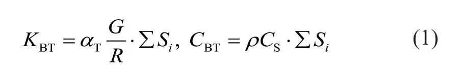
Normal boundary condition:

whereGandρare the shear modulus and mass density of the internal medium,respectively;CSandCPare the velocities of the shear wave and compression wave in the internal medium,respectively;and ∑Siis the boundary area represented by the finite element node connected to the viscoelastic artificial boundary.For the nodes on the surface boundaries,∑Si=L2;for the nodes on the edge boundaries,∑Si=L2/2;and for the nodes on the corner boundaries,∑Si=L2/4.Additionally,Lis the length of the finite element andRis the distance from the wave source to the artificial boundary.Because the wave sources in dynamic SSI problems are generally not single point sources,Ris typically designated as an average distance,andαTandαNare the artificial boundary parameters in the tangential and normal directions,respectively.Many numerical practices highlight the robustness of these artificial boundary parameters (Gu,2005).Reasonable results can be obtained when those parameters are selected within a given range of values.Guet al.(2007) recommends the parameter values that are shown in Table 1.

Table 1 Values of three-dimensional viscoelastic artificial boundary parameters αT and αN

3 Stability analysis method of explicit integration algorithms when using viscoelastic artificial boundaries

3.1 Stability analysis method based on subsystems

Explicit integration algorithms can be executed without solving coupled equations,leading to fewer calculation workloads and higher computationalefficiency.Thus,they are suitable for a dynamic analysis of large-scale complex systems.Numerical stability is the primary factor restricting the integral time steps in explicit calculations.Previous stability analyses of computing systems with artificial boundaries are generally based on overall numerical models or complex nodal systems composed of multiple rows or columns of nodes (Kamel,1989;Guan and Liao,1996).Because of the complexity of the objects of the study,the stabilities of those models are typically determined through numerical methods.However,due to the difficulty in obtaining uniform analytical stability criteria,the practicality of such methods is limited.

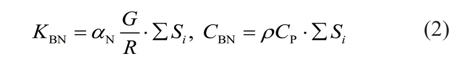
Liet al.(2020) summarized existing research on the stability of numerical integration methods for discrete models and came to the following conclusions: (1) the stability of the integration algorithm is controlled by the highest-order frequency of the numerical model (i.e.,the cutoff frequency) (Liu and Sharan,1995);and (2)the mode shape corresponding to the cutoff frequency typically presents staggered vibration of adjacent nodes.Considering a one-dimensional shear beam as an example,the vibration mode is shown in Fig.2.

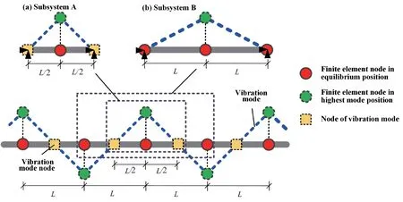
Fig.2 Schematic diagram of stability analysis based on local subsystems

Based on these conclusions,Liet al.(2020) proposed a method to estimate the stability of the overall numerical model based on localized subsystems.According to this method,for any finite element model,a local subsystem surrounded by adjacent nodes of the highest-order vibration mode can be extracted if the highest-order mode can be accurately determined.This is illustrated by substructure A of the 1D shear beam model,which contains one central node and two boundary nodes.The central node is the finite element node between two half elements.The two boundary nodes are the adjacent nodes of the highest-order vibration mode,which means these two nodes will remain stationary during the vibration that corresponds to the highest-order mode.By imposing constraints on the boundary nodes of this subsystem,which can ensure the same motions as the highest-order mode shape of the overall mode while performing a stability analysis,the stability condition of subsystem A can be obtained.Its condition is equal to the stability condition of the overall model.For situations in which the highest-order mode of the overall model cannot be accurately determined,several subsystems composed of adjacent elements,which can describe different localized characteristics of the overall model,can be extracted,and fixed constraints can be imposed on all boundary nodes of those subsystems (see subsystem B in Fig.2).Then,the stability conditions of all B-type subsystems can be obtained through theoretical analyses,whose lower limit is the upper limit approximation of the stability condition of the overall finite element model.

When using this method to analyze the stability of the internal calculation region of a model with viscoelastic artificial boundaries,an A-type subsystem can be applied to directly determine the corresponding stability condition.For boundary regions in which the influence of the artificial boundaries must be considered,it is difficult to directly determine the vibration mode corresponding to its cutoff frequency;thus,subsystem A is usually difficult to determine.In this case,B-type subsystems can be used for stability analyses.Compared to subsystem A,subsystem B is unrelated to the specific cutoff frequency of the model and its highest mode shape,and thus can be easily established and unaffected by the specific situation of the model.In this way,the stability problem of the overall finite element model is transformed into the stability analysis of a series of local subsystems composed of several elements.Next,by establishing the motion equations of the subsystems and,according to the explicit integration algorithms that are used,the analytical stability conditions of the local subsystems can be theoretically analyzed,which can be further applied to a stability judgment of the overall finite element model.Based on its strong operability and fewer limitations on the type of applied artificial boundaries and integration algorithms,this method likely has broad applications in the stability analyses of large-scale dynamic systems when considering complex artificial boundary conditions.

3.2 The explicit integration algorithm and stability judgment method,based on the spectral radius of the transfer matrix

Stability conditions are strongly dependent upon adopted numerical integration methods.To solve stability problems with viscoelastic artificial boundaries in practical engineering applications,we conduct a stability analysis based on the leap-frog scheme central difference method,which has been widely used in general finite element software,such as Abaqus.For other time-domain stepwise integration algorithms,the corresponding stability conditions can be obtained through similar procedures proposed in this study.

Based on the explicit integration algorithm used in this study,the time-domain recurrence formulae of the nodal motions in the 3D finite element model can be expressed as:

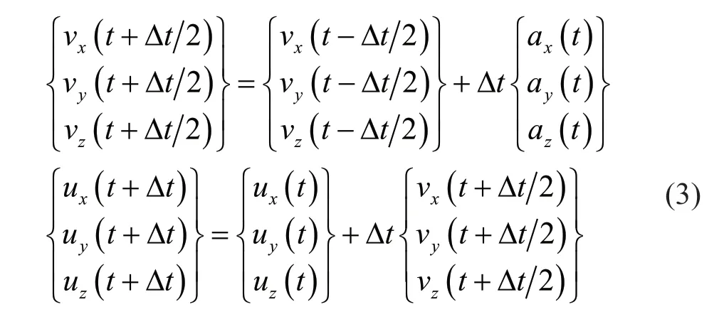
whereu,vandaare displacement,velocity and acceleration,respectively;tis time;Δtis the integration time step;and the subscriptsx,yandzdenote thex,yandzdirections in Fig.1.

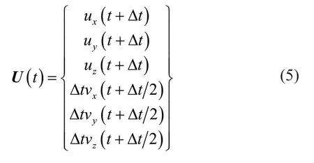
The motion equation of the discrete dynamic system can be rewritten based on the explicit integration scheme as follows:

whereAis the transfer matrix;Pis the vector of loads;and the vectorUconsists of the displacement,velocity,and acceleration of each node in the numerical system.The explicit integration algorithm used in this study is:

The stability condition of a specific numerical integration method is only related to the discrete space length and time steps,as well as the mechanical parameters of the calculation system,but it is not connected with load vectorP.The integration format is stable if the following conditions are met (Hughes,1983):

(1)ρ(A) ≤ 1,whereρ(A) is the spectral radius of transfer matrixA,ρ(A)=max|λi|,andλiis theith eigenvalue of transfer matrixA.For the 3D condition,i=1-6;

(2) IfAhas multiple eigenvalues,the moduli of those eigenvalues are all below 1.

Based on these theories and methods,the stability analysis of the explicit integration algorithm when using viscoelastic artificial boundaries can be decomposed into three steps: (1) select all types of subsystems that can describe the different localized characteristics of the overall finite element model;(2) establish the motion equations of each subsystem,deriving the corresponding transfer matrices based on the explicit integration algorithm,and solve the spectral radii;and(3) solve the stability conditions of each subsystem based on a constraint condition in which the modulus of the spectral radius should be below 1,and then select the strictest stability condition as the upper limit estimate of the maximum stable integral time step in the dynamic calculation.

4 Stability analysis of the explicit integration method when using viscoelastic artificial boundaries

In this section,the stability analysis of the explicit time-domain integration algorithm when using 3D viscoelastic artificial boundaries is presented.The stability conditions are closely related to the element size and physical characteristics of the computing system.When studying the stability of numerical integration algorithms,without losing generality,regular geometric models,homogeneous media,and uniform discrete grids are typically applied for modeling and analysis.For irregular grids or inhomogeneous media in practical applications,based on the minimum size of the finite elements and the different material parameters,we can calculate the stability conditions in different regions separately through the stability criterion introduced in this study,and then select the strictest stability condition to determine the maximum integral time step in the explicit dynamic calculation.

4.1 Subsystems of viscoelastic artificial boundaries

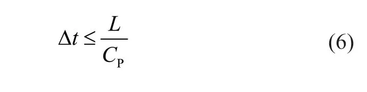
A schematic diagram of a discrete 3D near-field finite element model of semi-infinite space is shown in Fig.3.Without damping,the stability condition of the internal homogeneous domain in the central difference algorithm is given by Liet al.(2020):

When viscoelastic artificial boundaries are used in the explicit dynamic calculation,because it is difficult to determine the highest-order mode shape.B-type subsystems,as shown in Fig.2,should be used for stability analyses.Based on the different intercepted positions,the B-type subsystems containing artificial boundaries can be divided into three types: surface boundary subsystems,edge boundary subsystems and corner boundary subsystems,as shown in Fig.3.The motion equations and transfer matrices of those three types of subsystems will be established separately in the following section;subsequently,their stabilities in the explicit integration algorithm can be analyzed.

The local subsystems shown in Fig.3 are only composed of 3D brick elements and viscoelastic artificial boundaries (spring-damping systems).The physical parameters of the artificial boundaries are introduced in Eqs.(1) and (2).To establish the motion equations of those local subsystems,the stiffness matrix of a 3D isoparametric brick element should also be defined(Zienkiewiczet al.,2000):

Fig.3 Three-dimensional semi-infinite near-field finite element model and schematic diagrams of three types of boundary subsystems

where subscripts 1-8 denote the node numbers displayed in Fig.4.

The submatrices in Eq.(7) are given by:

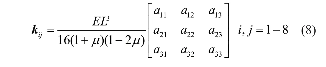
whereEis Young′s modulus;μis Poisson′s ratio;and:

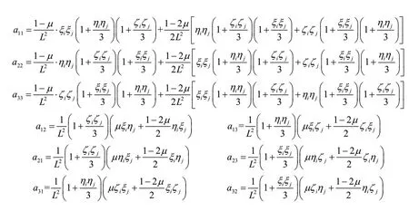
whereξ,ηandζare local coordinates in the FEM,ξi,j=±1,ηi,j=±1,ζi,j=±1,and subscriptsiandjdenote the node numbers shown in Fig.4.

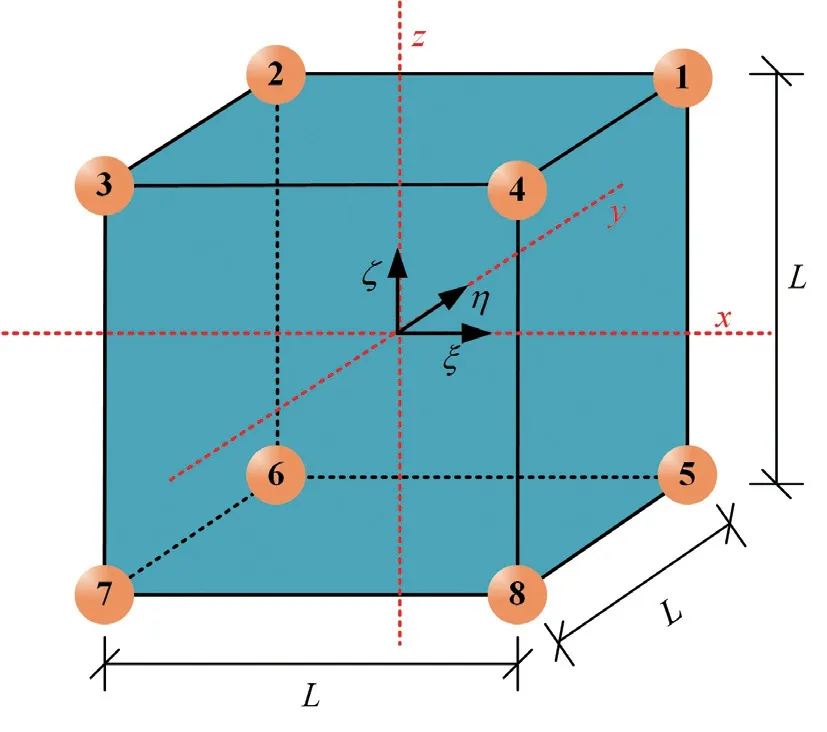
Fig.4 Schematic diagram of the three-dimensionalisoparametric brick element and the local coordinatesystem

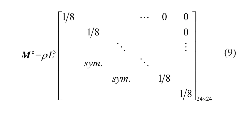
The concentrated mass model is used to establish the mass matrix of the 3D isoparametric brick element,which is given by:

4.2 Stability condition of surface boundary subsystem

The surface boundary subsystem is shown in Fig.5,in which only node 1 is free,and all other nodes,including the distal ends of the artificial boundaries,are fixed.The mass,damping and stiffness matrices of the surface boundary subsystem can be assembled based on the physical parameters of the viscoelastic artificial boundary given by Eqs.(1) and (2),and the element matrices of the 3D isoparametric finite element provided by Eqs.(7)-(9).Then,the motion equations of the surface boundary subsystem can be obtained:

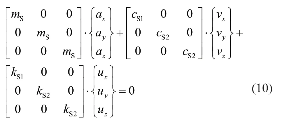
Fig.5 Schematic diagram of the surface boundary subsystem

where:

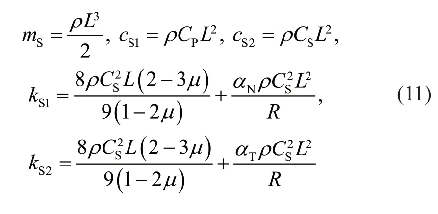
and the subscript S denotes the surface boundary subsystem.

By combining Eqs.(3) and (10),the transfer matrix of the surface boundary subsystem can be obtained:

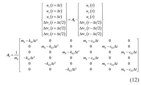
Next,the eigenvalues of transfer matrixAScan be solved:

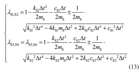
The stability criterion introduced in Section 2.2 can be equivalent to:

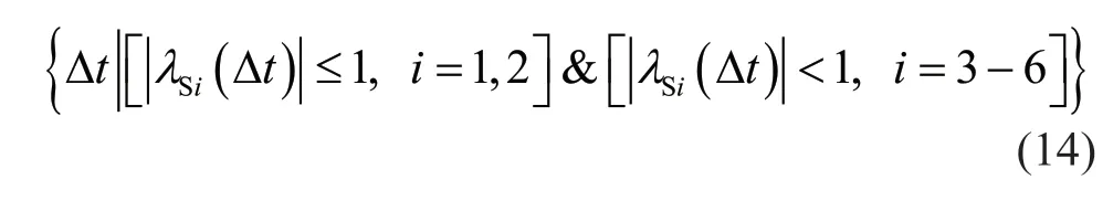
To solve Eq.(14),we can first solve the zero points of the following equation:

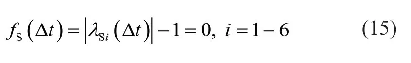
Considering that Δt≥0,the results of Eq.(15) are given by:

For the cases wherei=1,2 ori=3-6,the zero points shown in Eq.(16) divide the positive semiaxis of Δtinto two intervals.By examining whether the value of functionfS(Δt) is larger or below 0 when Δtis in different intervals,the ranges of Δtthat satisfy the stability conditions given by Eq.(14) can be determined based on the continuity of the function.

First,let Δtbe a small quantity greater than 0.Ignoring the high-order quantities o (Δt) in Eq.(13),we obtain:

By substituting Eq.(11) into the square root items of Eq.(17),the following equations can be gained:

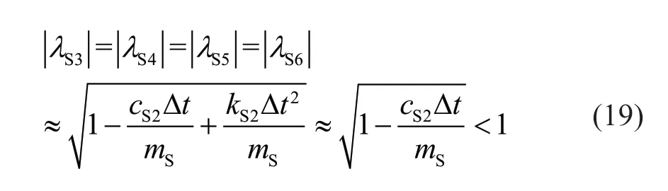
Because 0≤μ≤ 12,the value of the second equation in Eq.(18) is always negative;thus,λS3-λS6are all complex numbers,and their modules are:

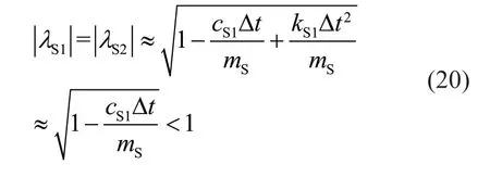
Additionally,when 0≤μ＜ 715,the value of the first equation in Eq.(18) is negative.In this situation,S1λandS2λare also complex numbers,and their modules are:

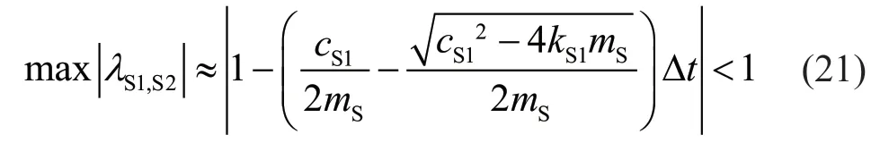
Additionally,let Δtapproach infinity.At this time,λSi,i=1-6 are all real numbers,and the maximum values of their modules satisfy:

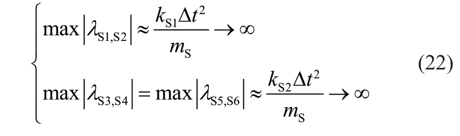
Based on the above analysis,and combined with the continuity of the function,the ranges of Δtthat satisfy the stability conditions given in Eq.(14) can be obtained as follows:

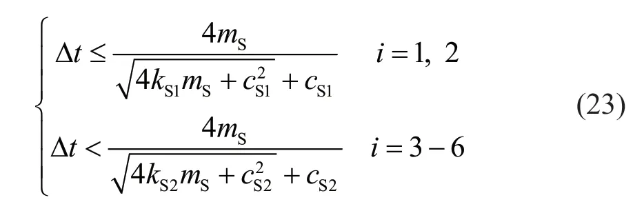
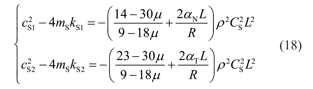
Equation (11) shows thatkS1＞kS2andcS1＞cS2;thus,the stability condition given by the first equation of Eq.(23) is stricter.Consequently,the stability criterion of the surface boundary subsystem can be arrived at:

By substituting Eq.(11) into Eq.(24),we get:

4.3 Stability condition of edge boundary subsystem

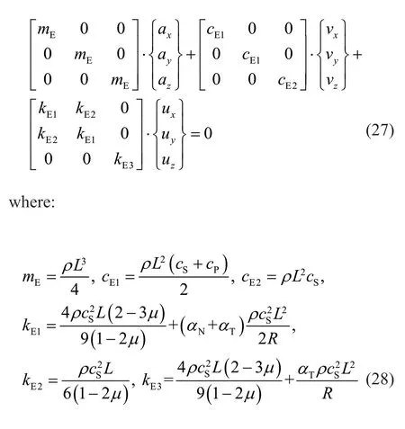
The edge boundary subsystem and its node numbers are shown in Fig.6.All nodes except node 1 are fixed.Assembling the stiffness,mass and damping matrices based on the node numbers,the motion equations of the edge boundary subsystem can be established:

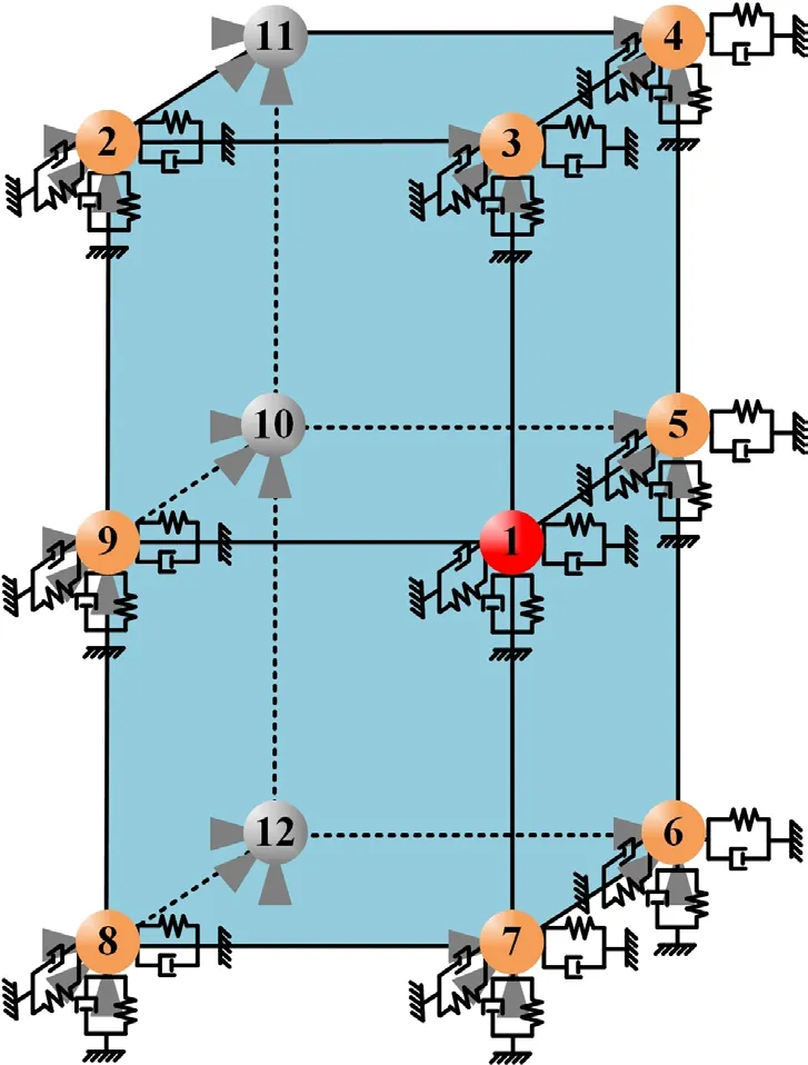
Fig.6 Schematic diagram of the edge boundary subsystem

and the subscript E denotes the edge boundary subsystem.

By combining Eqs.(3) and (27),the transfer matrix of the edge boundary subsystem can be obtained:

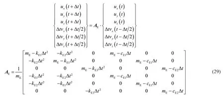
The eigenvalues of the transfer matrixAEcan be solved:

Next,we solve the zero points of equation-1= 0,i=1-6and obtain:

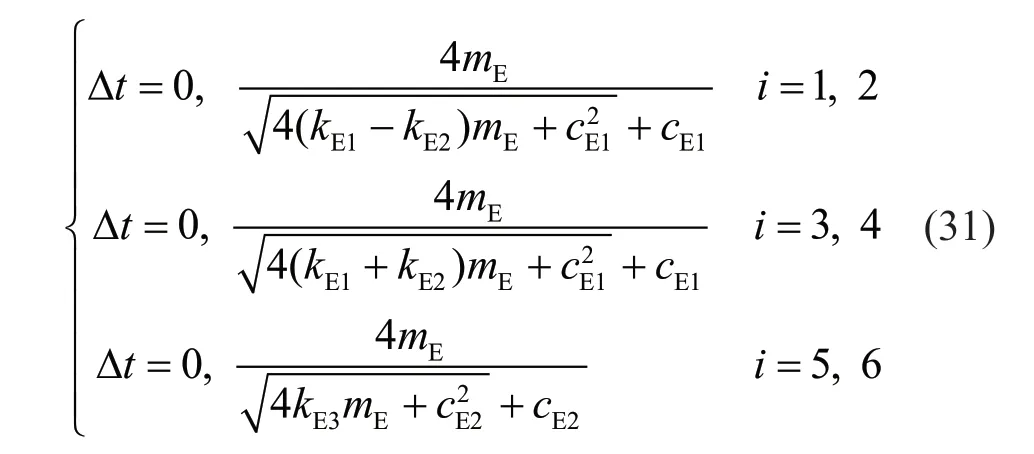
Based on the continuity of the function and the positions of zero points,and following a similar method presented in Section 3.2,the ranges of Δtthat satisfy the stability condition can be determined:

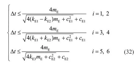
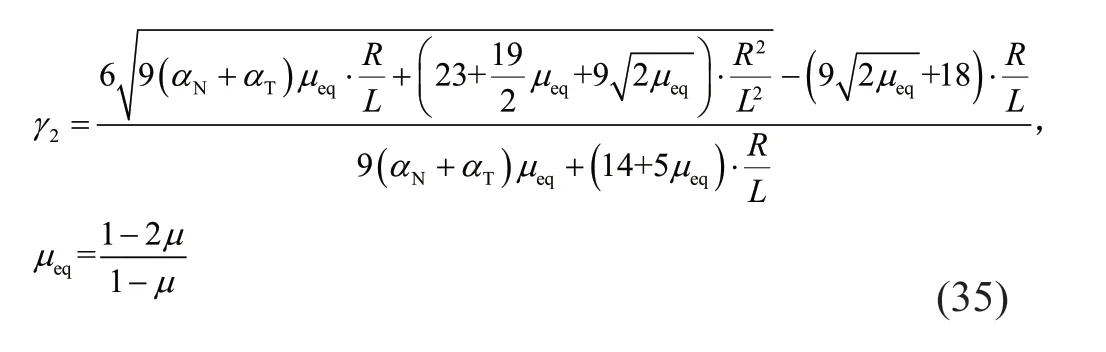
Equation (28) shows thatkE1＞kE3,kE2＞0 andcE1＞cE2;therefore,the second equation in Eq.(32) presents stricter conditions,and the stability criterion of the edge boundary subsystem can be finally determined:

By substituting Eq.(28) into Eq.(33),we obtain:

where:

4.4 Stability condition of corner boundary subsystem

The corner boundary subsystem and its node numbers are shown in Fig.7.Similar to the surface boundary subsystem and the edge boundary subsystem,all nodes except node 1 in the corner boundary subsystem are fixed.Through matrix assembly,the motion equations of the corner boundary subsystem can be established:

Fig.7 Schematic diagram of the corner boundary subsystem

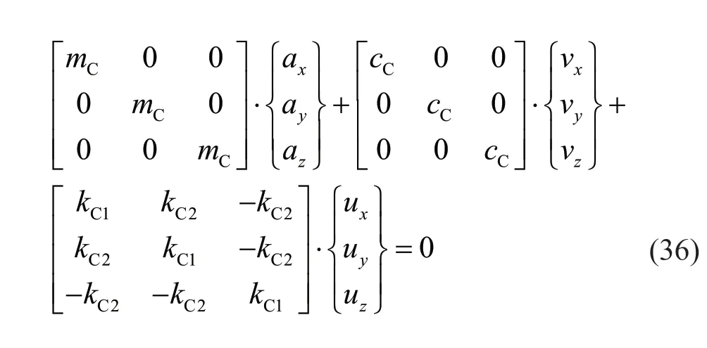
where:

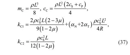
and subscript C denotes the corner boundary subsystem.

By substituting Eq.(3) into (36),the transfer matrix of the corner boundary subsystem can be obtained:

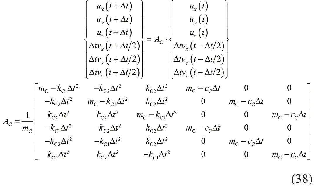
Then,the eigenvalues of the transfer matrixACcan be solved:

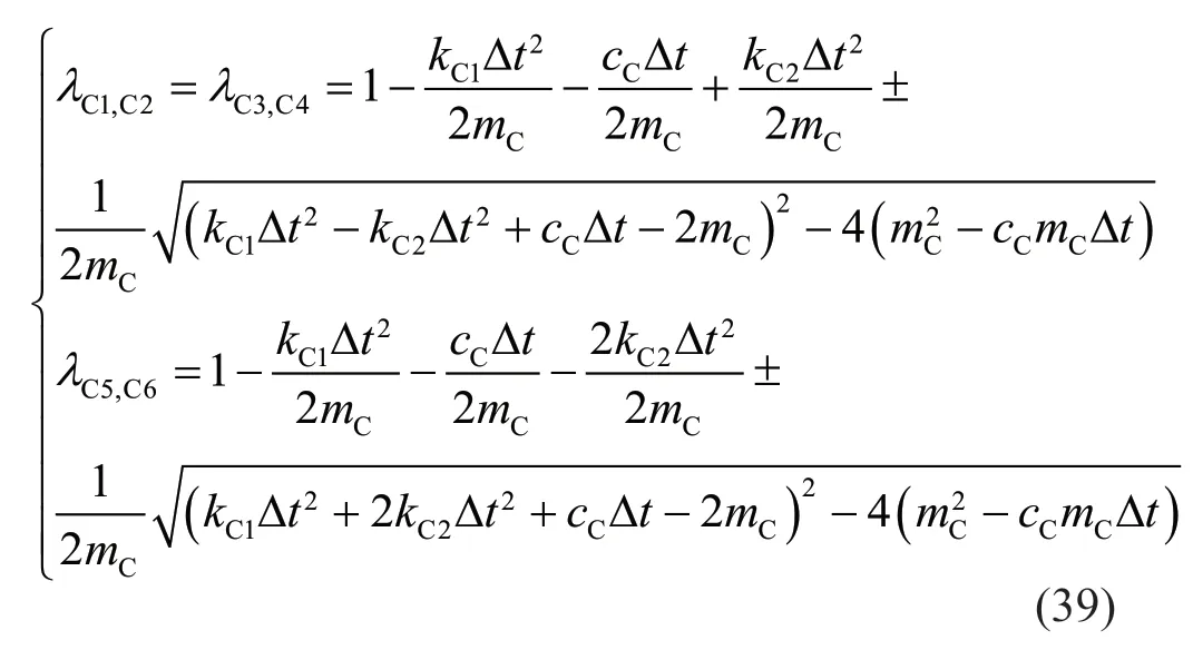
and the zero points of the equation-1=0i=1-6,can be calculated as:

Following a similar method presented in Section 3.2,the regions of Δtthat satisfy the stability condition can be determined:

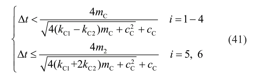
SincekC1,kC2andcCare all larger than 0,the stability condition of the corner boundary subsystem is controlled by the second equation of Eq.(41):

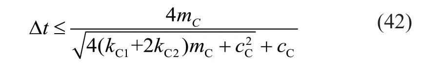
Substituting Eq.(37) into Eq.(42),we obtain:

4.5 Comparison of stability conditions

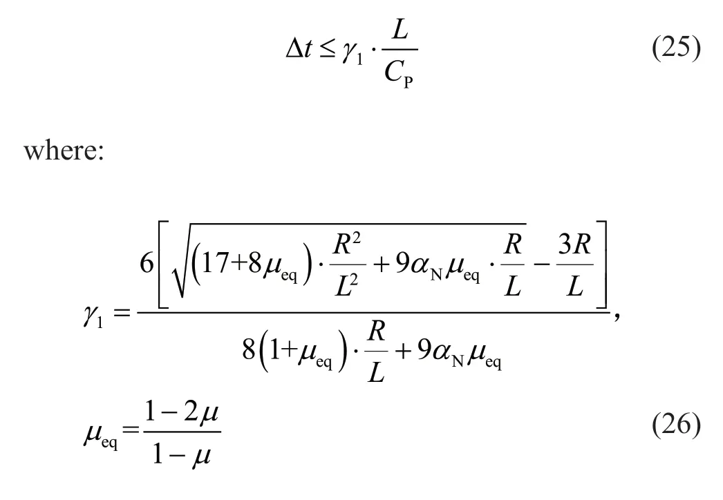
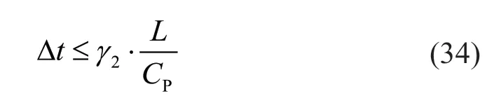
Next,we compare the stability conditions of the internal region,the surface boundary subsystem,the edge boundary subsystem,and the corner boundary subsystem.Based on Eqs.(25),(34) and (43),the stability conditions of the explicit integration algorithm when using viscoelastic artificial boundaries can be uniformly expressed as:

whereγis the global stability coefficient.

Equations (45),(26),(35) and (44) show that the stability coefficientsγ1,γ2andγ3of the surface,edge and corner boundary subsystems are all dimensionless.Additionally,those coefficients are only related to Poisson′s ratioμof the internal domain and the ratio between the distance from the wave source to the boundaryRand the length of the finite elementL.The variation in the stability coefficientγwithμandR/Lis now investigated,as shown in Fig.8.We then compare the distribution of the stability coefficientγalong with Poisson′s ratioμwhenL/Ris 1,5 and infinity,as well as the distribution of the stability coefficientγalong withR/Lwhen Poisson′s ratioμis 0.2,0.3 and 0.4.These comparisons are shown in Fig.9 and Fig.10,respectively.

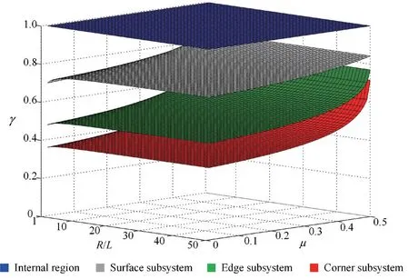
Fig.8 Comparison of stability conditions

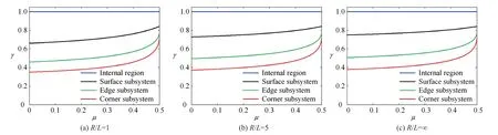
Fig.9 Variation in the stability coefficient γ with Poisson′s ratio μ under different R/L ratios

Fig.10 Variation in the stability coefficient γ with L/R under different Poisson′s ratios μ

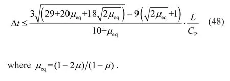
The results shown in Figs.8-10 show that the numerical stability conditions of the surface,edge and corner subsystems all become looser with an increase in Poisson′s ratioμ.With increasingR/L,the stability conditions of those subsystems first relax marginally and then remain basically unchanged whenR/Lis above 5.In addition,for arbitrary combinations ofμandR/L,the stability condition of the internal region is always the loosest.Due to the influence of the stiffness and the damping of the viscoelastic artificial boundaries,the stability conditions of the surface,edge and corner boundary subsystems are significantly stricter.Among these,the corner boundary subsystem presents the smallest stability coefficient in any case,indicating that the corner region controls the numerical stability of the overall model.Thus,its stability condition is the global stability condition of the explicit integration algorithm when using viscoelastic artificial boundaries,which can be expressed as:

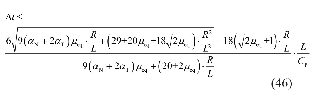
whereμeq=(1-2μ)(1-μ).

When the viscoelastic artificial boundaries and the central difference integration method are used for explicit dynamic analyses,based on the parameters of viscoelastic artificial boundaryαNandαT,the Poisson′s ratioμof the internal medium and the ratio between the distance from the wave source to the boundary and the length of the finite elementR/L,the maximum stable integral time step can be calculated through Eq.(46).

Additionally,to conveniently determine a stable integral time step,Table 2 provides the stability coefficients for several common situations.In general engineering problems,the following conditions are typically met:μ≥ 0.1 and≥ 5.Additionally,the stability conditions are known to loosen with increasingμandR/L.Therefore,in practical applications,the stability condition corresponding to the situation ofμ= 0.1 and=5,as shown in Eq.(47) can be used to obtain a conservative estimate of the maximum stable integral time step without complex calculations.The actual stability conditions are normally stricter than those calculated by the recommended stability coefficient,which further guarantees the reliability and reasonability of the proposed method.

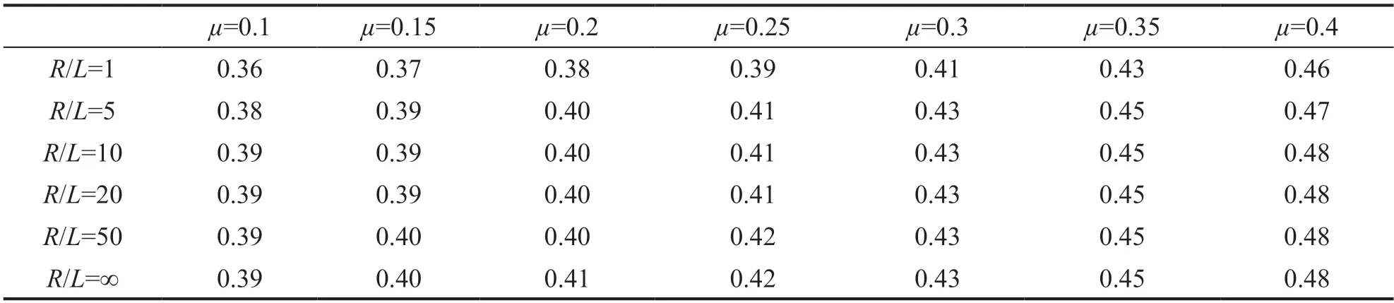
Table 2 Recommended stability coefficient γ

5 Stability condition of viscous artificial boundaries

The viscoelastic artificial boundary is a localized stress-type boundary condition derived based on the motions of two-dimensional cylindrical waves and threedimensional spherical waves.During the early study of artificial boundaries,the outgoing waves are usually assumed to be one-dimensional plane waves,and the localized boundary condition derived in this situation is the viscous artificial boundary.Because of its simplicity and convenience,viscous artificial boundaries are still widely used in wave propagation analyses.Compared to the viscoelastic artificial boundary,the viscous artificial boundary only consists of equivalent damping but no spring.Its damping parameters are identical to those of the viscoelastic artificial boundary.Namely,a viscoelastic artificial boundary can degenerate into a viscous artificial boundary when the equivalent spring is deleted,orRin the physical parameter equation of the viscoelastic artificial boundary tends to infinity.

Because of equivalent damping,the viscous artificialboundary also tends to tighten the stability conditions when using explicit integration algorithms.Considering that the viscous artificial boundary can be degenerated from the viscoelastic artificial boundary,the stability condition of the explicit integration algorithm when using the viscous artificial boundaries can be obtained by designatingRin Eq.(46) as infinity:

6 Verification of stability conditions

To verify the accuracy of the stability analysis,a wave propagation problem in a homogeneous half-space model is calculated using the general finite element software Abaqus.The numerical model is shown in Fig.11 (only three-quarters of the model is plotted for clear presentation).The size of the model is 100 m×100 m×50 m,and the mass density,shear wave velocity,compression wave velocity and Poisson′s ratio of the internal medium are 2000 kg/m3,200 m/s,374 m/s,and 0.3,respectively.Hexahedral isoparametric elements are used for finite element discretization with a mesh size of 1 m×1 m×1 m.Viscoelastic artificial boundaries are applied at the cutoff boundaries of the model,and the artificial boundary parametersαT=0.67 andαN=1.33 are used.A common sense approach to the numerical integral stability analysis is that the stability condition of a specific numerical integration method is only related to the discrete space length and the time steps,as well as the mechanical parameters of the calculation system,but is not connected to dynamic loads (Hughes,1983).Therefore,the derived numerical stability condition of the viscoelastic artificial boundary is unaffected by the specific load forms.To solely evaluate the effectiveness and accuracy of the derived stability condition when using viscoelastic artificial boundaries,we conducted a validation analysis through a simple internal source example.A concentrated pulse load with a duration of 0.1 s and an amplitude of 1×106N,as shown in Fig.12,is applied on the midpoint (pointA) of the ground surface.Observation pointsBandCare the point on the free surface and the point beneath pointA,whose distances to pointAare both 25 m.PointDis the corner point.Based on the abovementioned model parameters,the values of the stability coefficients and the maximum integral time steps in different regions of the numerical model can be calculated through Eqs.(6),(25)-(26),(34)-(35) and(43)-(44),which are denoted as the theoretical values,and the recommended value of the stability coefficient can be obtained by using Eq.(47).Those values of the stability coefficients and the maximum integral time steps are shown in Table 3.

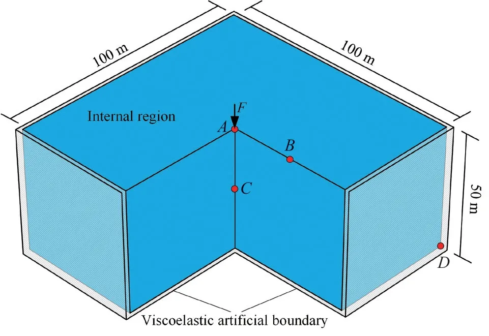
Fig.11 Schematic diagram of the 3D homogeneous half-space model

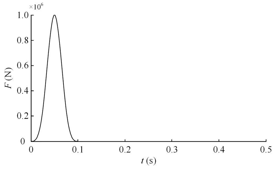
Fig.12 Time history of impulse load

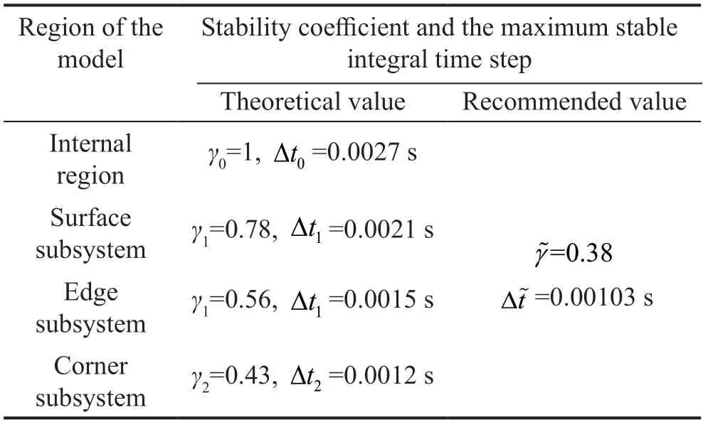
Table 3 Stability coefficients and maximum stable time steps of the 3D homogeneous model

Different fixed time steps are used to perform the explicit dynamic calculations,and their stability statuses are presented in Table 4.The displacement distributions of the models in the unstable cases are shown in Fig.13 and in the stable case in Fig.14.In addition,to verify the accuracy of the results calculated through the viscoelastic artificial boundaries,we conducted a comparative analysis on the presented example through an extended finite element model,whose cutoff boundaries are set as far as possible so that the false waves reflected by the cutoff boundaries will not reach the observation points.The accuracy of the results calculated by the extended finite element model is guaranteed by the finite element method and thus can be designated as numerically accurate solutions.The vertical displacements on pointsA,BandCwhen using the stable integral time step Δt=0.00103 s are compared with one another,and the results are given in Fig.15.Figure 16 shows a comparison of the vertical displacement time histories on the bottom corner (pointD) of the model with viscoelastic artificial boundaries under different fixed integral time steps.

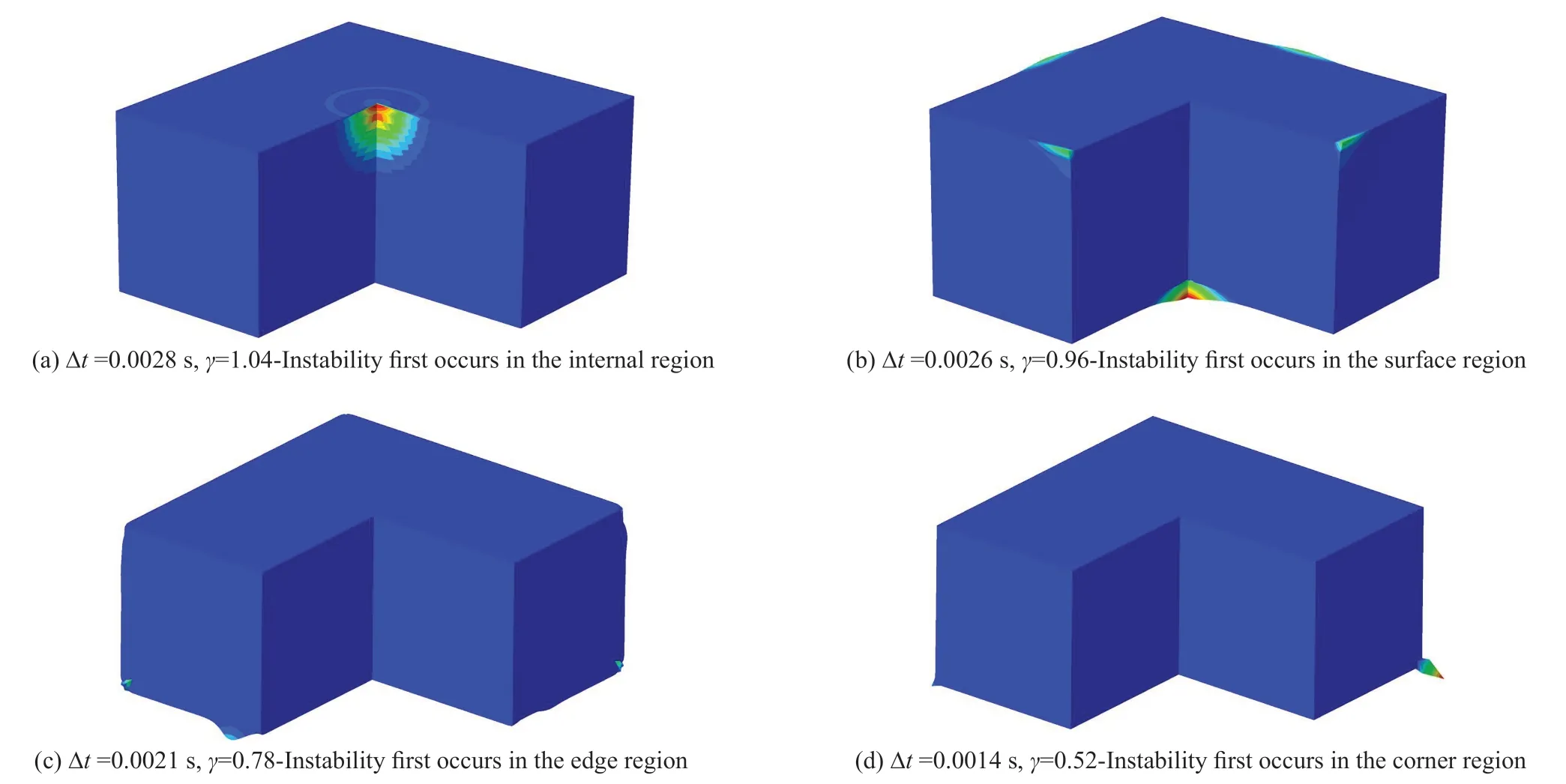
Fig.13 Unstable states of the 3D homogeneous half-space model

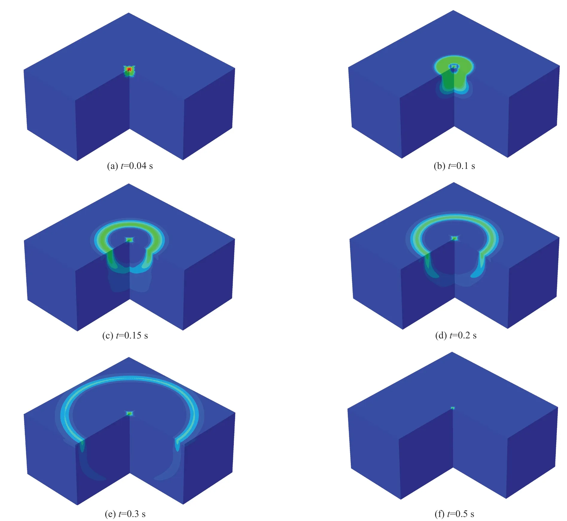
Fig.14 Displacement distributions in the 3D homogeneous half-space model when the integral time step is Δt=0.00103 s

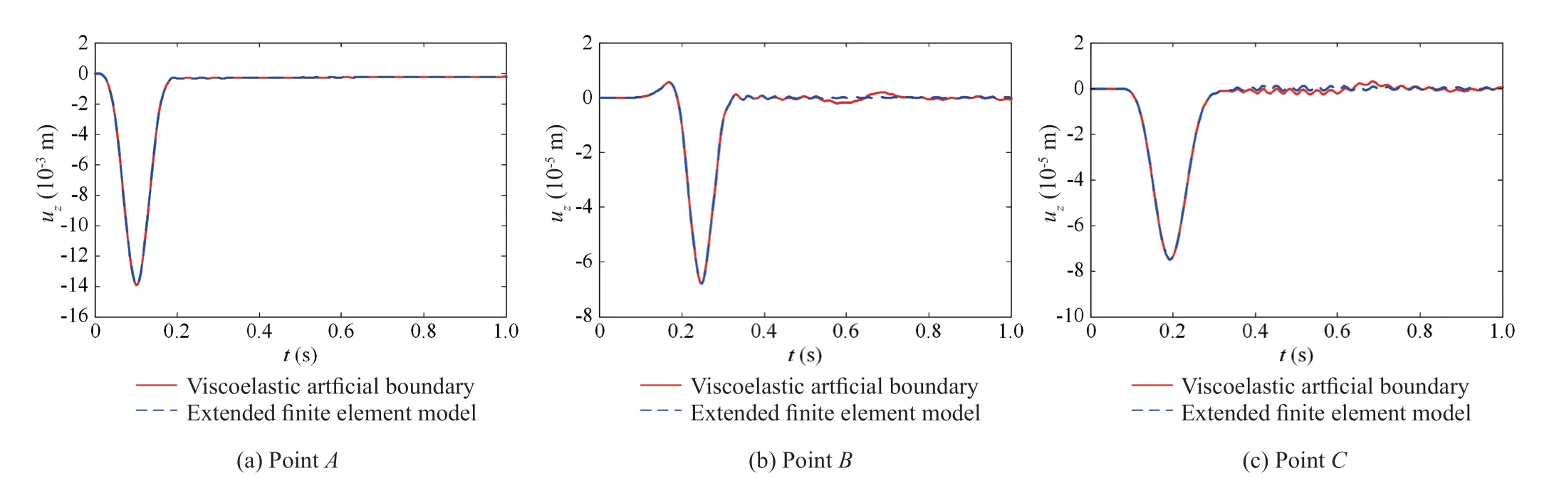
Fig.15 Comparison of vertical displacement histories calculated by the viscoelastic artificial boundaries and the extended finite element model when the integral time step is Δt=0.00103 s

Based on the results shown in Table 4 and Figs.13-16,together with the theoretical values and the recommended values of the maximum stable time steps in different regions given in Table 3,the following conclusions can be made: (1) the displacement wave fields calculated by the viscoelastic artificial boundary present nice agreement with those obtained from the extended finite element model,verifying the accuracy and effectiveness of this numerical technique for wave propagation simulation in an infinite domain;(2) the analytical stability conditions of the explicit integration algorithm when using the viscoelastic artificial boundaries presented in this study can accurately determine the stability state in the numerical calculation;(3) when the integral time step does not satisfy the stability conditions of the internal region,the surface boundary subsystem,the edge boundary subsystem or the corner boundary subsystem,instability will occur in the corresponding regions,as shown in Fig.13;(4) when the integral time step meets the stability condition of the corner boundary subsystem,the numerical calculation can be successfully completed,indicating that the stability of the explicit integration algorithm when using the viscoelastic artificial boundaries is controlled by the corner regions;and (5) because the recommended values of the stability coefficient are more conservative than the theoretical values,using the integral time steps determined by the recommended stability coefficient given in this study can ensure the successful completion of the explicit dynamic calculation.

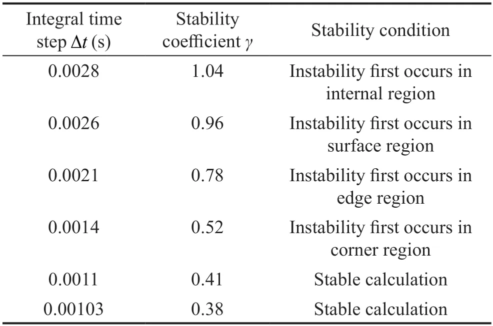
Table 4 Stability of the homogeneous model under different fixed time steps

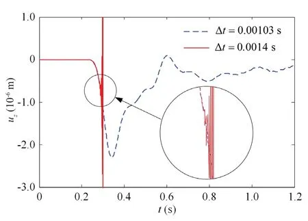
Fig.16 Vertical displacement time history of the corner point(Point D) in the 3D homogenous half-space model

7 Conclusion

This study focuses on the 3D viscoelastic artificial boundary,uses the stability analysis method based on the local subsystem to investigate its stability in the explicit integration algorithm,and verifies the accuracy of the stability analysis through numerical examples.The conclusions and results of this study are as follows:

(1) The analytical solutions of the stability conditions in the surface,edge,and corner boundary regions of the numerical model in the explicit time-domain stepwise integration algorithm when using viscoelastic artificial boundaries are derived.Additionally,when the viscoelastic artificial boundary degenerates into a viscous artificial boundary,we also derived the corresponding stability conditions.

(2) The numerical stability of a model with viscoelastic artificial boundaries is stricter than that of the homogeneous domain.The stability conditions of the artificial boundary regions are only related to Poisson′s ratioμ,the ratio between the distance from the wave source to the boundary and the length of the finite elementR/L,and the maximum stable time step of the internal regionL/CP.With an increasingR/Landμ,the stability conditions of the artificial boundary region tend to loosen.

(3) The stability of the overall model is controlled by the corner region.The global stability criterion of the numerical model with viscoelastic artificial boundaries is obtained,which can be applied to predict the stability status of the overall model in dynamic calculations.

(4) By analyzing the impact of different factors on the stability conditions,a conservative recommended value for the stability coefficient in the explicit integration algorithm when using viscoelastic artificial boundaries can be determined.In practical applications,this recommended stability coefficient can be directly used for estimating the maximum stable time step in the explicit dynamic calculation.

It is important to note that viscoelastic artificial boundaries are proposed based on the theory of FEM.Therefore,the derived stability conditions are only appropriate for determining the stable time steps in explicit dynamic FEM calculations.In addition,the numerical stability conditions are strongly dependent upon the adopted explicit integral methods.In this study,we conduct a stability analysis based on the leap-frog scheme central difference method,which has been used in general finite element software such as Abaqus.For other time-domain stepwise integration algorithms,one should derive the corresponding stability conditions following similar procedures.

Acknowledgement

This study is supported by National Natural Science Foundation of China (Grant Nos.52108458,U1839201),China National Postdoctoral Program of Innovative Talents (Grant No.BX20200192),the Shuimu Tsinghua Scholar Program (Grant No.2020SM005) and the National Key Research and Development Program of China (Grant No.2018YFC1504305).Financial support from these organizations is gratefully acknowledged.