Simplified lateral free field boundary based on a lumped mass system

Dong Zhengfang ,Kuo Chenyang ,Shi Chengli and Wang Junjie

1.Institute of Geotechnical and Rail Transport Engineering,Henan University,Kaifeng 475004,China

2.State Key Laboratory of Disaster Reduction in Civil Engineering,Tongji University,Shanghai 200092,China

Abstract: After reviewing the studies on the lateral artificial boundaries in dynamic soil-structure interactions,the free field boundary was theoretically analyzed in asymmetric-and symmetric-matrix forms.First,the lumped mass system was combined with viscous or viscoelastic elements to obtain a lumped mass-free field boundary.Second,typical examples were implemented using the finite element software ABAQUS.The incident shear wave was taken to be perpendicular to the bottom to verify the effectiveness of the lumped mass-free field under various sites: underground structures,uniform sites,and layered sites.Finally,the accuracy of the lumped mass-free field boundary was compared with those of the viscoelastic and roller boundaries on different calculation scales,soil damping ratios,structure sizes,and ground motion characteristics.Subsequently,the engineering design values for different damping ratios are given.The results show that the precision of the lumped mass-free field boundary was reasonable,and the operation was simple within the same engineering application.

Keywords: underground structure;artificial boundary;free field boundary;lumped mass system;interaction

1 Introduction

With the increasing utilization of underground space,dynamic soil-structure interactions have become the research focus.A building foundation is a semiinfinite space and the dynamic response characteristics of the buried and above-ground structures differ in multiple ways (Hashashet al.,2001).The numerical simulations of seismic responses in soil-structure dynamic interaction models must appropriately handle the semi-infinite space problem of the foundation and the input of ground motion.

In the earliest solution method in semi-infinite space,the truncated boundary was placed sufficiently far away that the reflected wave at the artificial boundary could not reach the region of interest (ROI).Even if the reflected wave reached the ROI within the calculation time,it would exhibit a negligible effect on the structural response (Altermanet al.,1970).To simulate the seismic response of an underground structure,a majority of researchers construct a finite near-field model,including the underground structure and the surrounding soil,as well as impose artificial boundaries.Wolf (1985) and Du (2009) applied the finite element method with an artificial boundary that extracts a finite region of soil mass near the ROI from the infinite volume of soil mass.Zhaoet al.(2017) ignored the scattering field and inputted only free field stress to simplify the input method.The free field response at the artificial boundary accounted for more than 90% of the total response.Based on this method,other researchers (Donget al.,2018;Pelekiset al.,2017;Rizzitanoet al.,2014;Tripeet al.,2013) adopted the constraint boundary method to realize a free field input at the artificial boundary.This approach reduced the modeling workload and obtained a satisfactorily accurate numerical calculation.At the artificial boundary,the outer traveling wave from the near-field finite field must enter the infinite field without reflection (Duet al.,2006).Therefore,the artificial boundary conditions must simulate the transmission of the scattering field and input at the artificial boundary to calculate the free field seismic response.

During the course of the past 40 years,artificial boundaries have been intensively and extensively researched.The main artificial boundaries are the transmitting boundary (Nakamura,2012),the viscous boundary (Lysmer and Kuhlemeyer,1969),the viscoelastic boundary (Liu and Lu,1998),the infinite element boundary,and the free field boundary.To realize a transmitting boundary,the scattered wave must be distributed to infinity,which requires an equal wave velocity governed by the one-way wave principle(Liaoet al.,1982).The transmitting boundary can be combined with the finite element method to improve numerical accuracy (Yang and Li,2012) but risks highfrequency oscillation instability and low-frequency drift instability (Konget al.,2005).The viscous boundary,first proposed by Lysmer and kuhlemeyer (1969),requires intercepting the ROI from the foundation and then setting a series of viscous dampers on the boundary surface.The viscous dampers simulate the radiation of scattered waves from the finite field of the foundation to the infinite field.A viscous boundary is stable at high frequencies,is easily applied in engineering (Lysmer and Kuhlemeyer,1969),and has a clear physical meaning,but is prone to low-frequency drift instability.The viscoelastic boundary,first proposed by Deeks and Randolph (1994),applies a remote fixed parallel springdamping system at the artificial boundary.Although this approach solves low-frequency drift instability of the viscous boundary (Deeks and Randolph,1994;Du and Zhao,2010),it requires different spring stiffness values.The viscoelastic boundaries provide high accuracy and are easily implemented with the use of finite element software.Accordingly,more recently they have been widely used and developed (Du and Zhao,2010;Nakamura,2012;Liuet al.,2005;Zhao,2009;Zhaoet al.,2015).For the two-dimensional viscoelastic artificial boundary element,Liet al.(2020) established the edge subsystem and corner subsystem,which can represent typical characteristics of the overall system.This is done by using the analysis method of transfer matrix spectral radius,which is based on the central difference format that is commonly used.In this way,they derive the analytical solutions of the stability conditions of the edge subsystem and corner subsystem.The idea of infinite elements was first proposed by Ungless in the 1970s (Ungless,1973),and the first infinite element method was developed in the 1980s (Zienkiewi and Bando,1985) for use in fluid wave analysis (Zhang and Zhao,1987).Chow and Smith (2010) extended the use of the infinite element to solid media.However,the method is only applicable to internal source problems,and external source incidents(such as seismic effects) require additional investigation.Free field boundaries were first proposed by Seedet al.(1975).The free field boundaries in commercial software were added for the first time to the UDEC and FLAC programs of Itasca (Carranza-Torres and Fairhurst,1999).Free field boundary conditions were achieved by a secondary development method on the ABAQUS platform.Such free field boundaries reduce the workload of the model in solving the free field and are practical from an engineering perspective.Based on multi-directional transmitting and viscous-spring artificial boundary theories,Xuet al.(2012) proposed a new artificial boundary model for absorbing stress waves in a saturated soil foundation,with dynamic analysis.

Joyner and Chen (1975) and Bouckovalas and Papadimitriou (2005) derived the equivalent load of the artificial boundary under viscous boundary conditions in a one-dimensional model with seismic wave inputs.Based on the theoretical analysis of Joyner and Chen(1975),Yasuiet al.(1995) proposed a method that handles the oblique incidence angles of ground motion.Liuet al.(2006) proposed a wave method suitable for viscoelastic boundaries,which converts the input ground motion into an equivalent seismic load at an artificial boundary.The wave method can be used to obtain the equivalent input seismic load on the artificial boundary,which is then applied as the seismic-energy input to a soil-structure model.Previous studies (Zhaoet al.,2013;Joyner and Chen,1975;Bouckovalas and Papadimitriou,2005;Liu and Lu,1998) have confirmed the accuracy of the wave method,but the calculation is complicated.By deducing another form of equivalent input seismic loads in the finite element model,Liuet al.(2019) proposed a new seismic wave input method.In this new approach,by imposing the displacements of the free wave field on the nodes of the substructure,which is composed of elements that contain artificial boundaries,the equivalent input seismic loads are obtained through dynamic analysis of the substructure.Wolf (1989)proposed a free field boundary method that obtains free field responses in soil columns and converts them into boundary traction forces that act on the truncated boundary of a finite element model.However,the free field boundary method requires simultaneous step-bystep calculations in three calculation regions,thereby incurring a large calculation cost.

To avoid these problems,this study proposes a free field boundary that requires only ground motion input at the bottom of the model,based on the free field boundary theory and the lumped mass system.Calculations of the free field and equivalent input load are not required;rather,one simply inputs the ground motion at the bottom of the model.The influence of the artificial boundary location,soil damping ratio,structure scale and input ground motion on the lumped mass-free field boundary also is studied for comparison.

2 Theoretical analysis

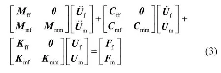
The free field boundary admits an automatic lateral ground motion.The free field boundaries of the symmetric and asymmetric matrix forms are shown in Fig.1.

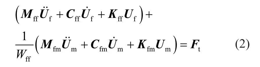
Generally,the motion equation of the free field and the master model can be written as follows (Nielsen,2006,2014):

whereWffis the width of the free field,andWmmis the width of the master model.Mff,Cff,andKffare the free field mass,damping,and stiffness matrix entries,respectively.Mmm,Cmm,andKmmare the mass,damping,and stiffness matrix entries of the master model,respectively.Mfm,Cfm,andKfmare the corresponding coupling matrix entries of the master model free field,andMmf,Cmf, andKmfare the corresponding coupling matrix entries of the free field to the master model.

Generally,a free field boundary condition is obtained using one of two methods.The first method modifies the matrix equation into an asymmetric form such thatMfm,Cfm,andKfmare0.The second method expands and arranges Eq.(1) as follows:

AsWffapproaches infinity,the second term in Eq.(2)approaches 0.By substituting Eq.(2) into Eq.(1),we obtain

This matrix equation is symmetric.Neither result is directly usable in the existing software.This paper proposes the following methods to avoid the secondary development of these equations.

2.1 Lumped mass free field boundary

The free field can be realized by settingWff.Viscous or viscoelastic elements can absorb the scattering wave.As an example,we consider the viscous element shown in Fig.1.To solve the large grid-number problem after discretization,a certain width of the soil on both sides of the main model was simplified as a series of lumped mass nodes connected by springs and dampers.The soil mass of the free field was replaced by the lumped mass system to simulate the free field of the original soil mass(Zhuang and Chen,2017).This simplification satisfies the requirements of a free field boundary while reducing the number of discrete meshes.

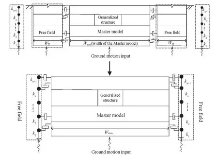
Fig.1 Model of the free field boundary

Theoretically,the lumped mass free field boundary provides an effect like that provided by the infinite field.A propagating wave is not reflected from the artificial boundary.In the numerical simulation,the lateral viscous or viscoelastic element will absorb the energy of the scattered wave,reduce wave reflection,and improve numerical accuracy.

2.2 The wave input method

For a vertically incident shear wave,pure shear motions are performed at any position in the calculation model and in the lumped mass system as a free field.If any micro unit is selected from the plane model,it will be in a pure shear state.Its stress state is shown in point A in Fig.2,andτrepresents shear stress.In the tangential direction of the artificial boundary on both sides,shear stress must be input;this stress factor can be provided by using the roller bearing with vertical constraint and horizontal freedom,and its bearing reaction force will be equal to the required input shear stress,as shown in pointBin Fig.2.Therefore,only the normal free field input on both sides is considered for a vertically incident s-wave.The vertical constraint and horizontal free roller boundary can be used to input the tangential stress in a tangential direction.

Fig.2 Wave inputs at the lumped mass free field boundary

As an example,consider viscoelastic elements in the normal direction.At boundary nodeAof the artificial boundary,denote the free field displacement vector as

,the velocity vector of the free field as,the spring coefficient of the viscoelastic element asKa,and the damping coefficient asCa.The force vector acting on the node in the master model can be given as follows:

whereAais the affected area around the node.WhenKa=0,the viscoelastic element becomes a viscous element.

3 Numerical verification

3.1 Numerical example

The lumped mass free field boundary was validated using a typical example in the ABAQUS finite element software.The parameter settings of the viscous and viscoelastic elements were obtained from Lysmer and Kuhlemeyer (1969) and Liu and Lu (1998),respectively.The lumped mass free field boundaries of the viscous and viscoelastic elements are expressed as free fields A and B,respectively.

The accuracies in the free fields A and B were evaluated at the viscoelastic boundary.The error was defined by the following three measures:

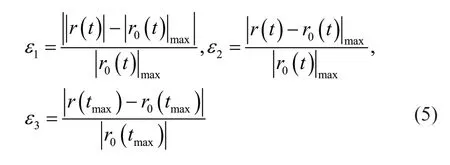
wherer0(t) andr(t) are the responses of the benchmark model and the lumped mass free field boundary,respectively,tmaxis the corresponding time at|r0(t)|max,and |*|maxis the maximum absolute value of “*”.

According to the definition of error,ε1is the relative error between the absolute value ofr(t) maximum and the absolute value of the benchmark model response maximum,ε2is the relative error between the absolute value of the maximum value of the time process of the difference betweenr(t) andr0(t) and the maximum value of the benchmark model response,andε3is the relative error between the value oftmaxtimer(t) and the maximum response value of the benchmark model.

The example was divided into three working conditions.Under working condition 1,the site was uniform,and the model settings are as shown in Fig.3(a).The model parameters were set as follows: site size=10 m × 10 m,shear wave velocity=170 m/s,unit weight=19 kN/m3,Poisson′s ratio=0.30.The ground motion input was a pulse wave.Under working condition 2,the site was a layered site,and the site parameters are listed in Table 1.TheB/Hwas 1.2,ground motion input was an El Centro wave,and the lumped mass width of the lumped mass system was 200000 m (proven to meet the requirements).Under working condition 3,the structure was underground,the field parameters are listed in Table 1,and the model settings are as shown in Fig.3(b).The structural parameters were set as follows: width=12 m,height=10 m,wall thickness=1 m,concrete density=2600 kg/m3,elastic modulus=32.5 × 109Pa,Poisson′s ratio=0.2.The four-node plane strain elements are used for both soil and underground structures,in which a 1 m × 1 m uniform grid is used for soil and a 0.25 m ×0.25 m uniform grid is used for underground structures.To consider the interaction between the soil and the rectangular concrete structure,a feature binding is adopted.The input wave is an El Centro wave,and the width of the lumped mass system was temporarily considered to be 200 kilometers (proven to meet the requirements).The ground motion parameters are those shown in Fig.4.

Fig.3 Schematics of the structural model

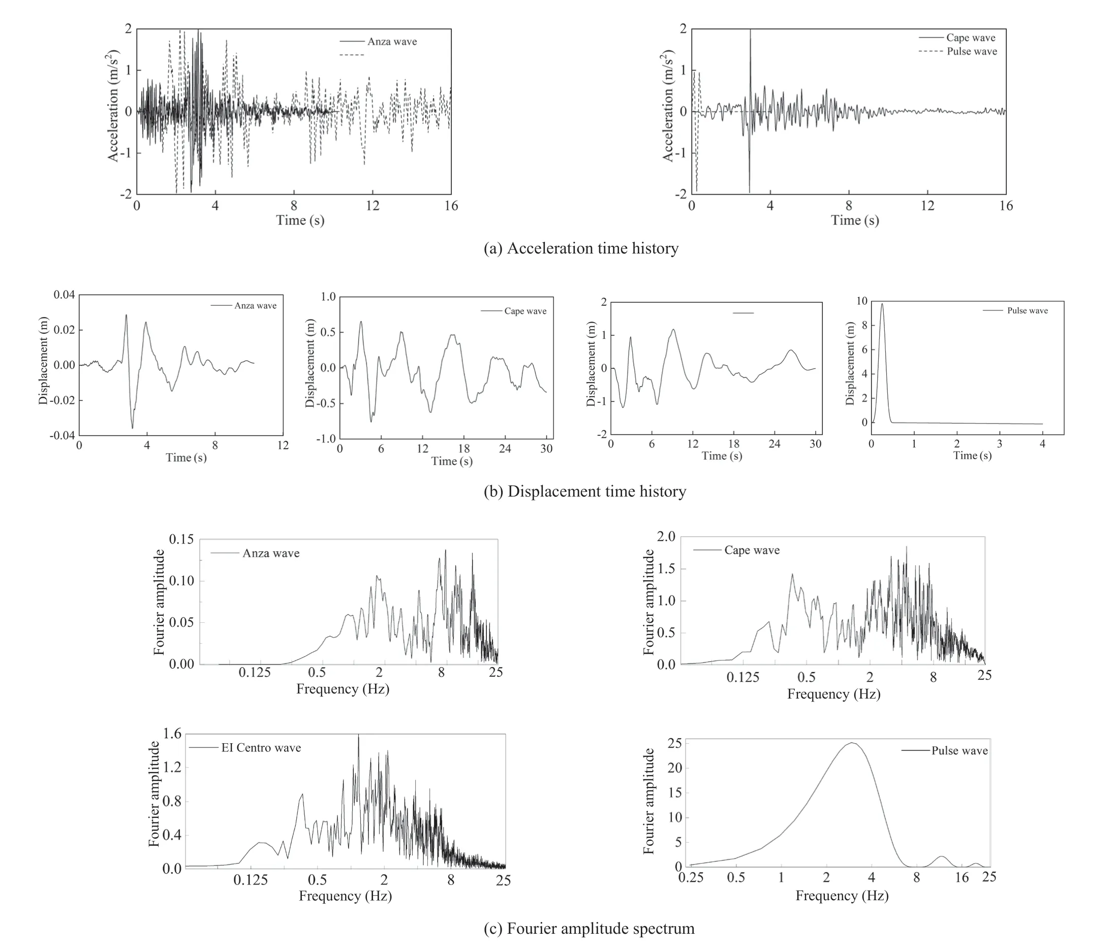
Fig.4 Ground motion parameters

Soil mass does not need to be infinite,but in principle the larger the value,the better.In the numerical calculation,if the value of the lumped mass system is too large,and the value of the matrix equation formed by the lumped mass system will be far greater than that formed by the master model,which is easy to form the“ill-conditioned matrix”,so that the calculation cannot be carried out.Therefore,in the numerical calculation,the free field width should have a reasonable range to ensure a smooth outcome.

After numerical calculation,we found that the influence of the value width of the lumped mass system on free field A and the free field B is basically the same,so that they may be replaced by each other.WhenBf/L=20000,the three errors are basically stable.(Bfis the width of the lumped mass system,Lis the width of the underground structure.)

3.2 Result analysis

The displacement time histories at the top and bottom of the soil layer were extracted under condition 1 to verify the accuracy of the centralized free mass field boundary.The results of various boundary conditions are compared in Fig.5.

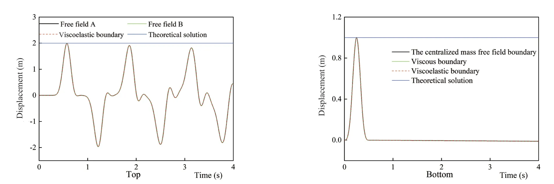
Fig.5 Time histories of the displacements at the top (left) and bottom (right) of the soil layer

The displacement time histories were identical at the lumped mass free field boundary and the viscoelastic boundary.This result validates the input method of the lumped mass free field boundary.

The error under each working condition was calculated from the average displacements at the top,middle,and bottom of the soil layer.As shown in Fig.6,the errors generated by the lumped mass free field and viscoelastic boundaries were almost zero under working conditions 1 and 2 and were non-zero but small under working condition 3.

4 Analysis of the influence factors of the lumped mass free field boundary

In an aseismic design,the main concern is the seismic response of the structure.According to Saint-Venant′s principle,the specific conditions at the boundary will only slightly affect the seismic response of the structure,provided that the boundary of the virtual calculation is sufficiently far from the structure.However,calculation time is increased when the virtual boundary is far from the structure.Therefore,the virtual boundary must be appropriately set in numerical calculations regarding the internal seismic response.The factors affecting the error introduced by the lumped mass free field boundary are analyzed below.

4.1 Working conditions

To generalize the results,an analysis was performed in soil layers at two depths (25 m and 64 m).The parameters of the 25-m and 64-m soil layers are listed in Tables 1 and 2,respectively.The setting range of the lateral boundary was discussed in the planar situation.Roller boundary (horizontal free,vertically constrained),viscoelastic boundary,free field A and free field B are used for a lateral boundary.The calculation model of the roller boundary is shown in Fig.2 (absorbing boundary and lumped mass system at both sides without two sides).The calculation model of the free field is shown in Fig.2 (it is the free field with the viscous absorbing boundary,and the free field with the viscoelastic absorbing boundary can be paralleled with spring).The bottom boundary is assumed to be rigid.

Table 2 Physical parameters of the 64-m soil layer

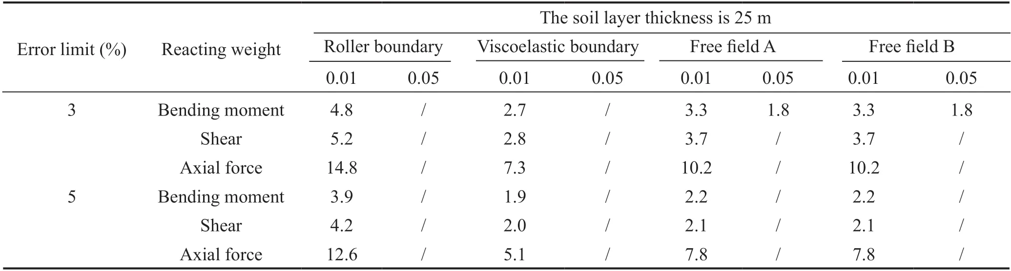
Table 3 B/H values satisfying error ε1

Table 4 B/H values satisfying error ε2

When the width of the calculation model isB≥ 8000 m,the lateral virtual boundary slightly affects the seismic response of the underground structure.Therefore,the lateral boundary is set as the roller boundary in the model withB=8000 m.

The accuracy of the model was evaluated for different width-to-thickness ratios of the soil layer under different conditions of the roller boundary,viscoelastic boundary,the lumped mass free field boundary A with a viscous absorbing boundary,and the lumped mass free field boundary B with a viscoelastic absorbing boundary.The damping ratio,structural scale,and ground motion characteristics were also varied.Displacement and internal forces results were evaluated under the three working conditions.The displacements of three nodes(a,b,and c) were compared,and the standard error of three nodes was computed.The positions are shown in Fig.3(b).The errors in the axial force,shear force,and bending moment were calculated at the top and bottom elements of the structure side wall.

4.2 Influence of calculation scale

TheB/Hratios were set to 1.2,3.6,6.0,10.8,and 19.0 in the 25-m soil layer,and 0.5,1.2,3.6,6.0,and 19.0 in the 64-m soil layer.The ground motion was an El Centro wave incident vertically from the bottom.Peak acceleration was uniformly adjusted to 0.2 g.The remaining parameter settings are given in Section 3.1.The errors in the soil displacement and structural internal forces were calculated as mentioned in Section 4.1.The calculated errors in the displacement responses of the 25-m and 64-m soil layers are shown in Fig.7,and the corresponding errors in the internal force responses of the structure are shown in Figs.8 and 9,respectively.The solid and dotted lines in these figures denoteε1andε2,respectively.The error results at the viscoelastic boundary were obtained from the literature (Wanget al.,2019).

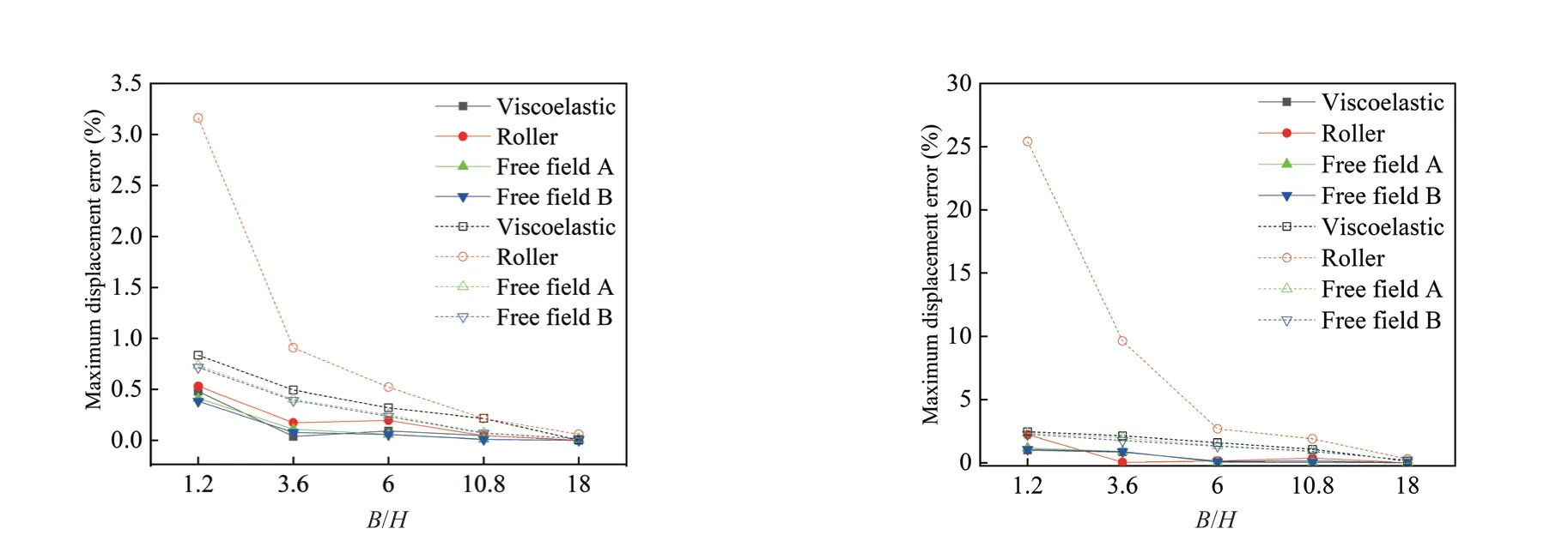
Fig.7 Calculation errors of displacement response in the 25-m (left) and 64-m (right) soil layers

As seen in Fig.7,ε1andε2decreased with increasingB/H,andε2was larger thanε1.In the 25-m layer soil,ε1was less than 1% atB/H≥ 3.6 in the viscoelastic boundary,free field A,and free field B cases,andε2was less than 1% atB/H≥ 6 in the roller boundary case.In the 64-m soil layer,bothε1andε2were less than 1% atB/H≥ 6 in the viscoelastic boundary,free field A,and free field B cases,but in the roller boundary case,ε2is less than 1% only whenB/His large.

Fig.8 Calculation errors in the structural internal force responses of the 25-m soil layer

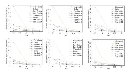
Fig.9 Calculation errors in the structural internal force responses of the 64-m soil layer

As theB/Hincreased,the internal force errorsε1andε2decreased non-monotonically and monotonically,respectively (Figs.8 and 9).In the 25-m soil layer,ε1was less than 1% atB/H≥ 6 in the viscoelastic boundary,free field A,and free field B cases and atB/H≥ 10.8 in the roller boundary case.Meanwhile,ε2was less than 1%atB/H≥ 6 in all four boundary cases.In the 64-m soil layer,ε1was less than 1% atB/H≥ 6 in all four boundary cases andε2was less than 1% atB/H≥ 19.Generally,the errors were almost identical in the free field A and free field B boundary cases.The accuracies after applying the free field A and free field B boundaries were lower than those obtained after applying the viscoelastic boundary but higher than those obtained after applying the roller boundary.The application of the free field boundary is helpful for reducing the numerical error from that of the roller boundary.

4.3 Influence of damping ratio

The width-to-height ratio was varied asB/H=3.6 and 6.0 in the 25-m and 64-m soil layers to evaluate the influence of soil damping ratio in the master model with different horizontal calculation widths.The soil damping ratio was varied as 1%,3%,5%,7%,10%,and 15%.The displacement responses of the 25-m and 64-m layer soils in the different boundary cases are compared in Fig.10.The solid and dotted lines are the results ofB/H=3.6 and 6.0,respectively.

As seen in Fig.10,increasing the soil damping ratio gradually decreased the calculation error,but the decrease was not necessarily monotonic.At a damping ratio of 1%,ε1was less than 1% in all the boundary cases.At damping ratios of more than 5%,the errorε2was less than 1% in the viscoelastic boundary and free field A and free field B boundary cases,but the roller boundary case required a larger damping ratio to achieveε2＜ 1%.Generally,the error values were almost identical after applying them to the free field A and free field B boundaries.At a given damping ratio,the free field A and free field B boundaries achieved slightly lower accuracy than was the case for the viscoelastic boundary but higher accuracy than the roller boundary.Applying the free field boundary is helpful for improving calculation accuracy when compared with that obtained by applying the roller boundary.

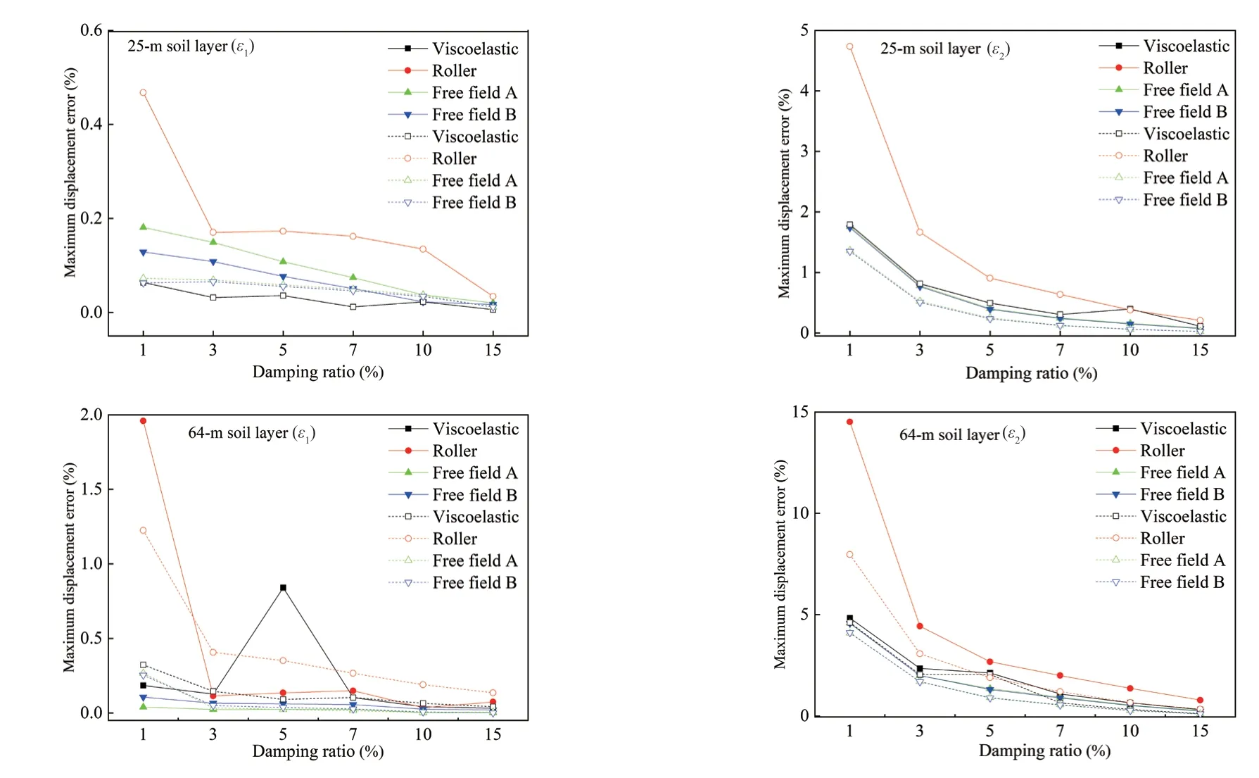
Fig.10 Calculation errors in the displacement responses

Figures 11 and 12 plot the internal force responses of the 25-m and 64-m layer soils,respectively,for different soil damping ratios in the different boundary cases.Increasing the soil damping ratio gradually decreased the error in the internal force response.To achieve the same small error,a greaterB/Hwas required for large structures when compared to that of small structures.The internal force error was higher atB/H=3.6 than that atB/H=6.0.In general,the Free Field A and Free Field B boundaries yielded errors between those of the roller and viscoelastic boundaries.Applying the lumped mass free field boundary is helpful for improving numerical accuracy.

4.4 Influence of structure scale

The structure size was varied as 50 m × 30 m (a large structure) and 12 m × 10 m (a small structure) to understand the influence of the underground structure scale on the calculation width of the master model.The soil was 64 m deep,and its damping ratio was 5%.The width-to-height ratio was varied asB/H=3.6 and 6.0.The calculated errors in the displacement responses and internal force reactions in these cases are compared in Figs.13 and 14,respectively.Along the horizontal axis of these figures,the small structures with the viscoelastic boundary,roller boundary,free field A,and free field B are denoted as working condition types 1,2,3,and 4,respectively.The large structures with the corresponding boundaries are denoted as working condition types 5,6,7,and 8,respectively.

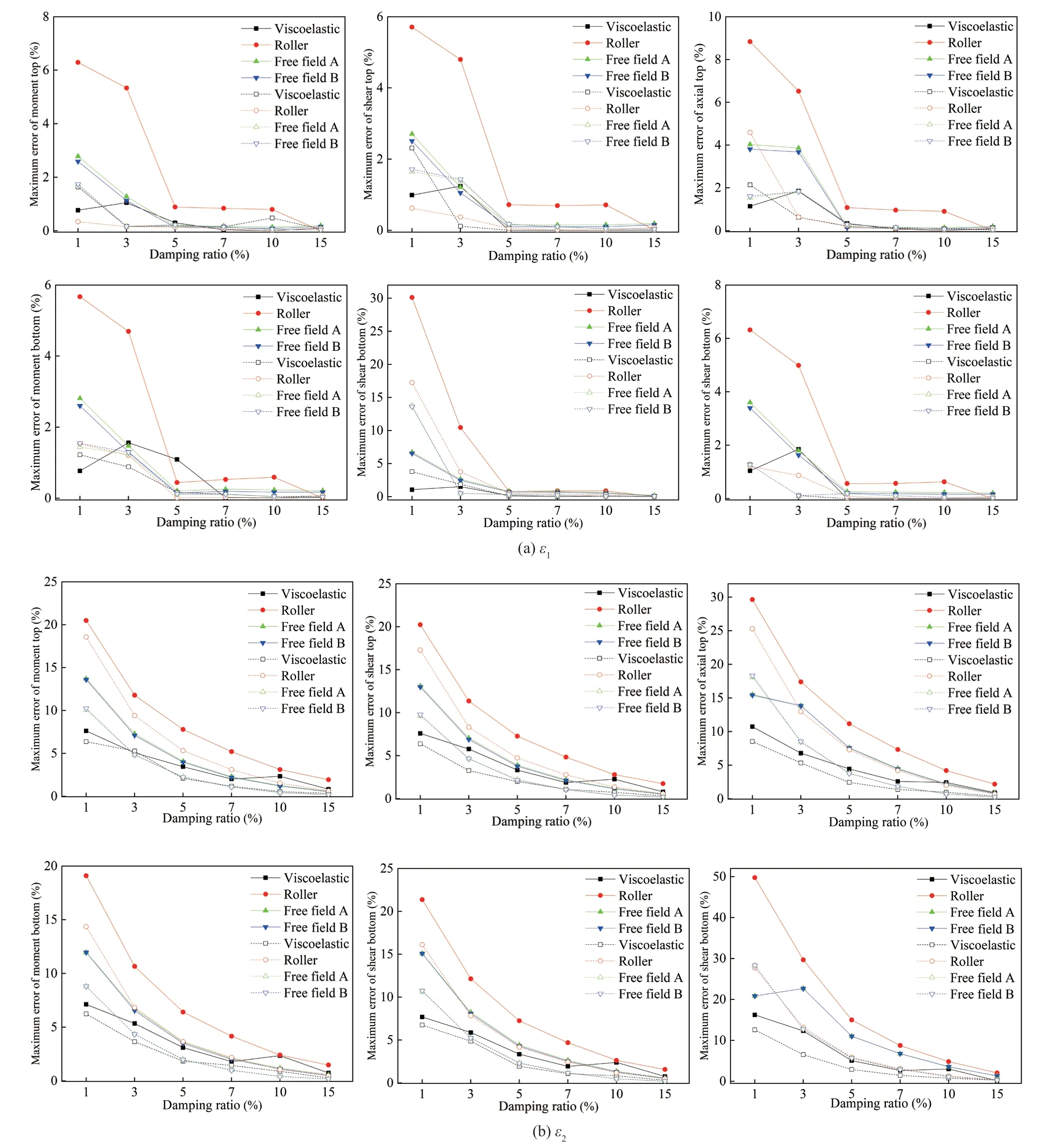
Fig.11 Calculation errors in the internal force responses of the 25-m soil layer

As shown in Figs.13 and 14,the size of the underground structure considerably influenced theB/Hat which a given error was reached.Under a given condition,the error was larger in the large structure when compared to that of the small structure.To obtain the same small error,a largerB/Hwas required in the large structure when compared to that of the small structure.The free field A and free field B boundary cases achieved larger error than the viscoelastic boundary case but smaller error than the roller boundary case.The error values in the free field A and free field B cases were largely consistent.Applying the free field boundary is helpful for improving calculation accuracy when compared to that of the roller boundary.

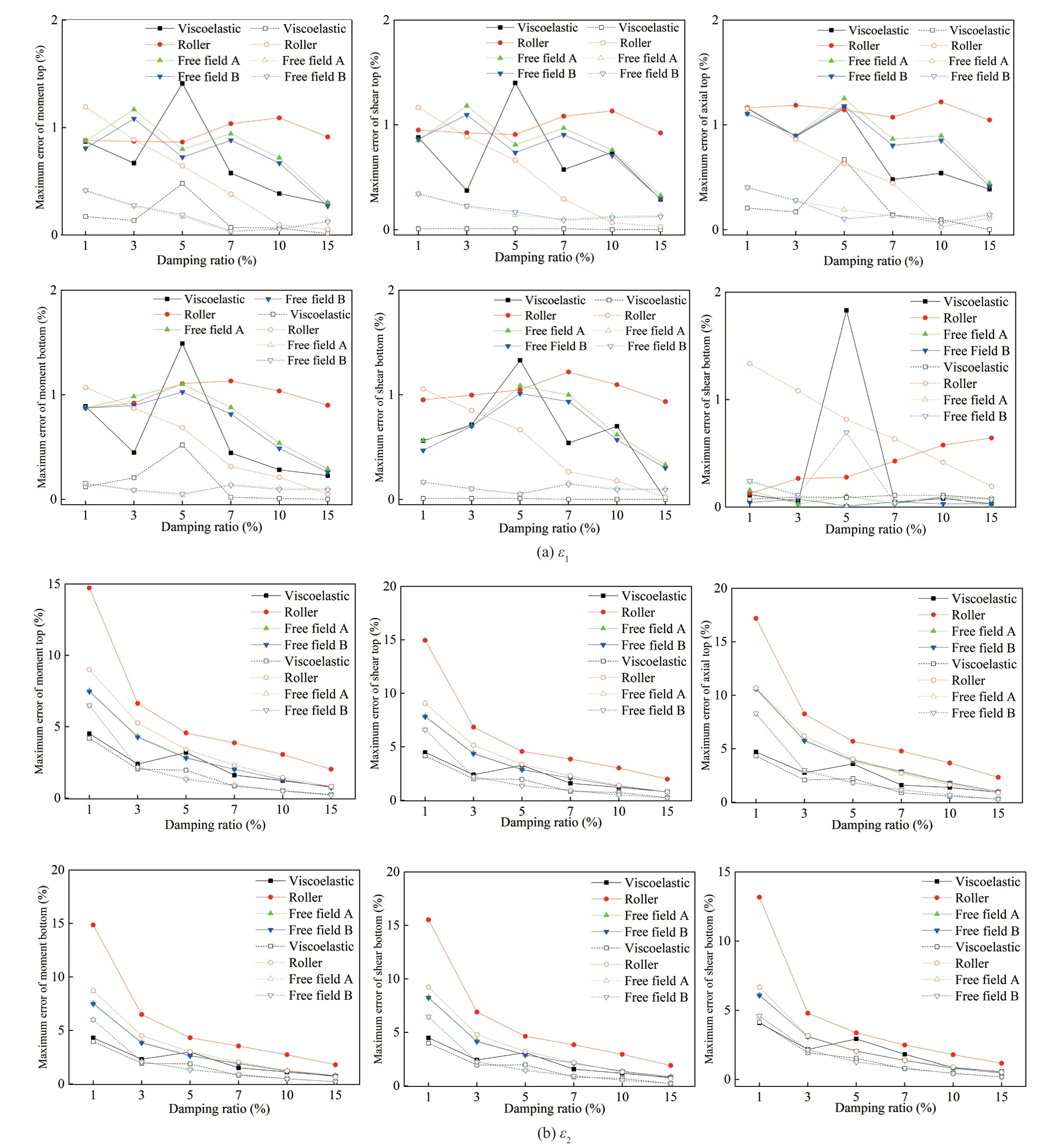
Fig.12 Calculation errors in the internal force responses of the 64-m soil layer

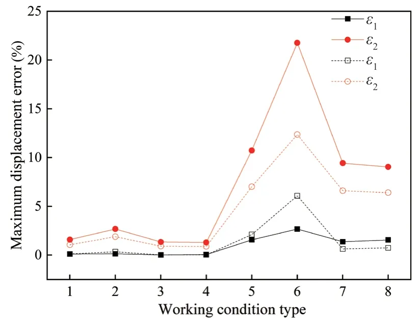
Fig.13 Calculation errors in the displacement response

4.5 Influence of ground motion characteristics

We selected three strong earthquakes records with different characteristics (different peaks,durations,and frequency spectra) and one pulse wave to study the influence of seismic characteristics on the calculated width of the master model.The soil layer was 64 m deep,and its damping ratio was 5%.The width-to-height ratio was varied asB/H=3.6 and 6.0.The El Centro,Cape,and Anza waves were denoted as ground motions 1,2,and 3,respectively.The errors in the displacement reactions and internal force responses under the various conditions are displayed in Figs.15 and 16,respectively.

As shown in Fig.15,the characteristics of the ground motion influenced the calculation error and the error in the artificial boundary cases.The errors in the viscoelastic boundary,free field A,and free field B cases were increased by the discretized form of ground motion 3.Meanwhile,the error in the roller boundary case was increased by the dispersion of ground motion 3 and the pulse wave.In general,the calculation error was lower atB/H=6 than that atB/H=3.6.The calculation accuracy was slightly lower in the free field boundary case than that in the viscoelastic boundary case but was higher than that in the roller boundary case.The errors in the free field A and free field B cases were very similar.Thus,higher accuracy can be achieved by applying free field boundaries when compared to that achieved by applying roller boundary conditions.

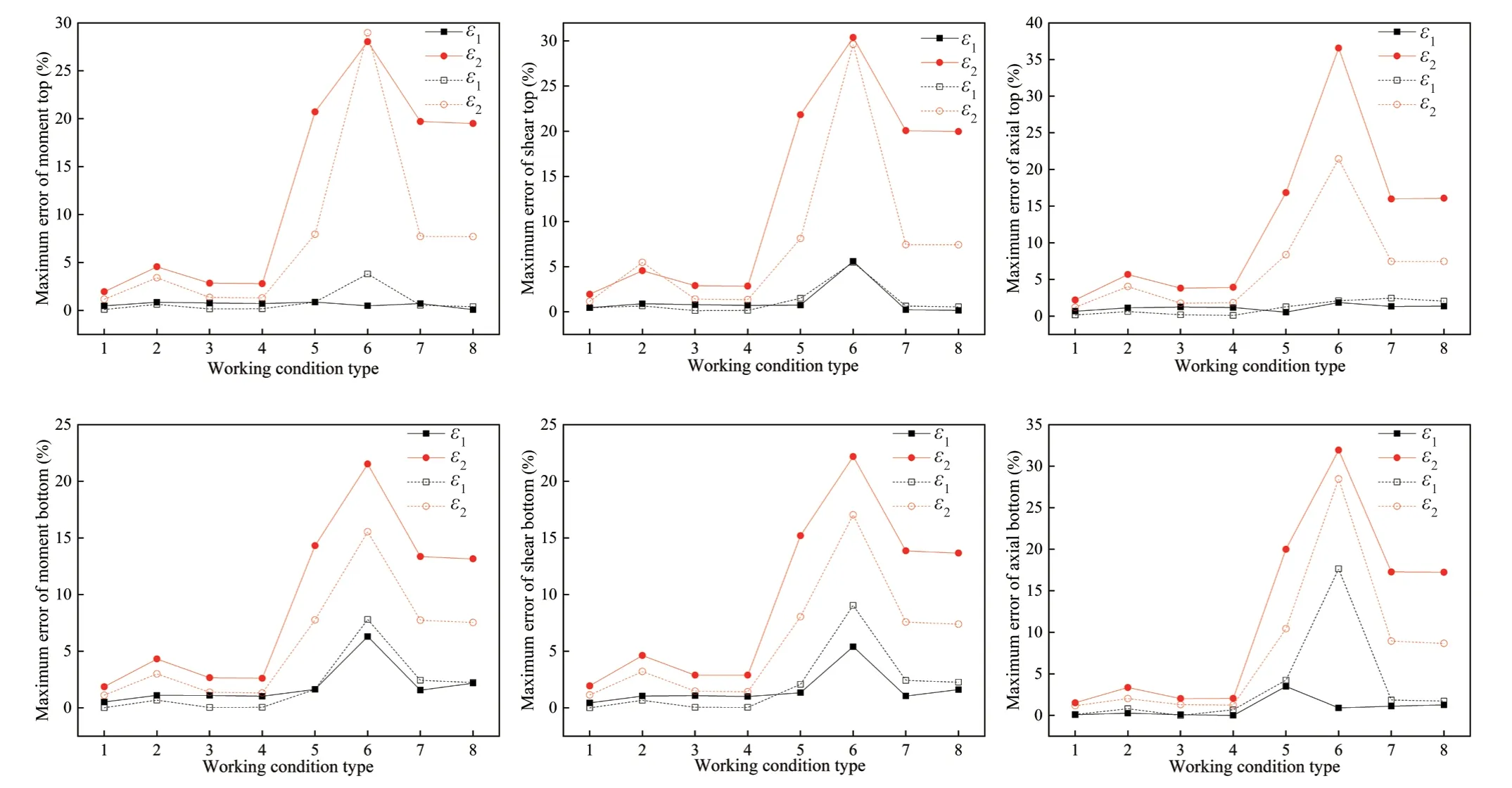
Fig.14 Calculation errors in the internal force responses

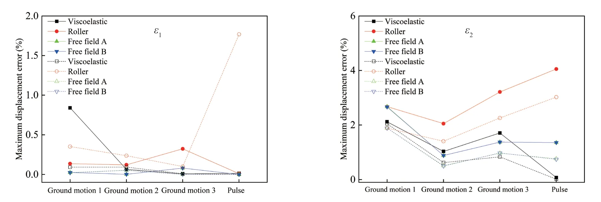
Fig.15 Errors in the displacement reactions

As shown in Fig.16,the errorε1was similar atB/H=6 and 3,but the errorε2was smaller atB/H=6 than that atB/H=3.Different ground motion characteristics yielded different responses.When selecting different seismic loads in seismic calculations,theB/Hvalue should satisfy the most unfavorable ground motion load.The roller boundary produced a larger dispersion than the other boundary types.In general,the errors were very similar in the free field A and free field B cases.The free field boundary achieved slightly lower accuracy than that achieved by the viscoelastic boundary but higher accuracy than that achieved by the roller boundary.

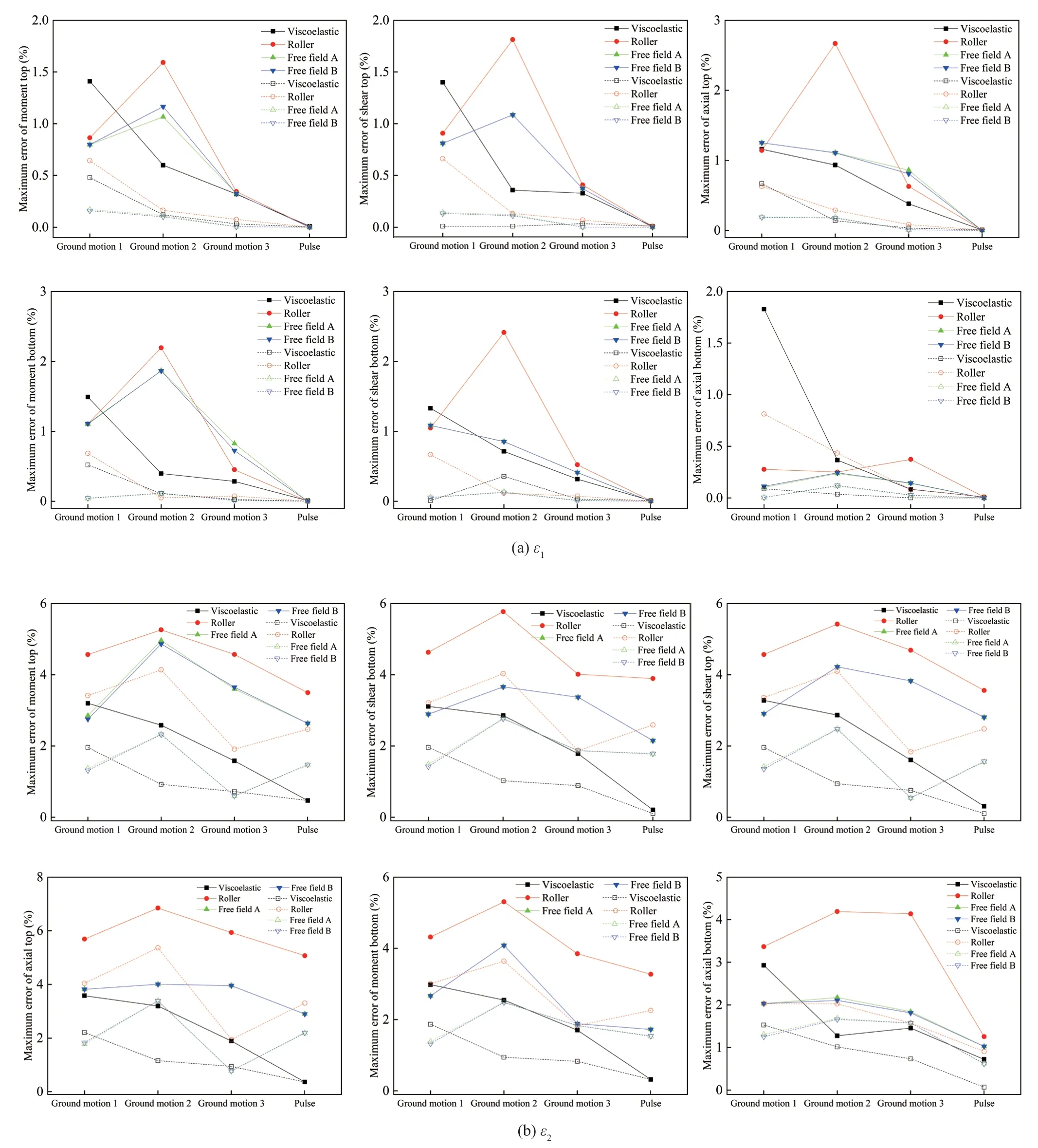
Fig.16 Errors in the internal force reaction

The higher accuracy of the lumped mass free field boundary compared to the other boundaries can be explained as follows.At the free mass boundary of the lumped mass,the absorbing boundary in one direction is set at the roller boundary and the absorbing boundary in one direction is set less than at the viscoelastic boundary.Therefore,the energy of the reflected wave at the lumped mass free field boundary is higher than that at the roller boundary but lower than that of the viscoelastic boundary.

5 Value of B/H in engineering design

It is impossible to accurately calculate the response of the structure in engineering design owing to the large number of uncertain factors.Therefore,a certain degree of accuracy must usually be satisfied in engineering design.This accuracy requirement is determined by the relative error of the maximum response,which is usually 3%-5%.Therefore,theB/Hvalue that meets a certain accuracy requirement for seismic calculation can be determined by use of the interpolation method.No larger calculation model is required.

The minimumB/Hvalues were obtained by linear interpolation under error criteria of 3% and 5%.The engineering designB/Hrequirements for 25-m and 64-m soil layers are shown in Tables 3 and 4,respectively.The solidus “/” in Tables 3 and 4 indicates that the calculated errors atB/H≤ 1.2 andB/H≤ 0.5,respectively,are less than the error control values.The values of 0.01 and 0.05 are the damping values.

Tables 3 and 4 show that the roller boundary requires a largerB/Hthan do other boundaries to achieve the same interpolation error.A damping ratio of 1% requires a largerB/Hthan that required by a damping ratio of 5%.Also,a higherB/His required for a 3% interpolation error than that required for a 5% interpolation error.DifferentB/Hvalues are usually required for different structuralresponse error indicators (such as bending moment,shear,and axial force).The numerical calculation should consider the required error index.Usually,the axial force error is large;therefore,theB/Hvalue satisfying the accuracy of the axial force error is considered the most unfavorable working condition.The requiredB/Hvalues were generally identical in the free field A and free field B cases.Free field A is recommended for conventional problems because its setting is less complicated than that of free field B.The requiredB/Hat the side boundary was larger in the lumped mass free field boundary (free field A and free field B) cases than that in the viscoelastic boundary case and smaller than that in the roller boundary case.

6 Conclusions

This paper theoretically analyzed the free field boundary in a symmetric matrix form using the finite element software ABAQUS.The accuracy of the approach was verified via the use of typical examples.Concluding remarks are given below.

· The lumped mass free field boundary has the same effect as the viscoelastic boundary in the free field analysis but exerts a slightly different effect from the viscoelastic boundary in the field with an underground structure.

· By enlarging the calculation model,the errors generated by the roller boundary,the viscoelastic boundary,and the lumped mass free field boundary can be reduced.By increasing the damping ratio,the errors generated by these boundaries and the required scale level of the calculation can be reduced.The larger the structural scale,the larger will be the calculation scale required in all boundary cases.The error in the soil layer reaction is dependent upon ground motion characteristics.

· The requiredB/His larger at a 1% damping ratio when compared with that at a 5% damping ratio.TheB/Hthat results in the same small error usually differs for different structural reaction error indexes (such as the bending moment,shear,and axial force).In numerical calculations,the required error index should be selected at the most unfavorableB/Hvalue.TheB/Hrequired at the side boundary was larger in the lumped mass free field boundary case than that of the viscoelastic boundary case but smaller than that of the roller boundary case.

· Accuracy was higher in the lumped mass free field boundary case than that of the roller boundary case and lower than that in the viscoelastic boundary case.The lumped mass free field boundary is highly stable.

Generally,the viscoelastic boundary requires a higher theoretical basis than is the case with other boundary types or a complex calculation process,but results in a high degree of accuracy.When applying the lumped mass free field boundary proposed in this study,ground motion only needs to be input to the bottom of the calculation model.The centralized free field boundary has a transparent physical meaning and can easily be realized with existing finite element software.Therefore,its applicability is guaranteed.