Mapping soil erodibility in southeast China at 250 m resolution:Using environmental variables and random forest regression with limited samples

Zhiyuan Tian,Feng Liu,Yin Liang,Xuchao Zhu

State Key Laboratory of Soil and Sustainable Agriculture,Institute of Soil Science,Chinese Academy of Sciences,Nanjing,210008,China

Keywords:Soil K factor Predictive soil mapping Machine learning Uncertainty

A B S T R A C T Soil erodibility(K factor)mapping has been accomplished mainly by soil map-linked or geo-statistical interpolation.However,the resulting maps usually have coarse spatial resolution at a regional scale.The objectives of this study were a)to map the K factors using a set of environmental variables and random forest(RF)model,and b)to identify the important environmental variables in the predictive mapping on a regional scale.We collected 101 surface soil samples across southeast China in the summer of 2019.For each sample,we measured the particle size distribution and organic matter content,and calculated the K factors using the nomograph equation.The hyperparameters of RF were optimized through 5-fold cross validation(mtry=2,ntree=500,p=63),and a digital map with 250 m resolution was generated for the K factor.The lower and upper limits of a 90% prediction interval were also produced for uncertainty analysis.It was found that the important environmental variables for the K factor prediction were relief,climate,land surface temperature and vegetation indexes.Since the existing K factor map has an average polygonal area of 6.8 km2,our approach dramatically improves the spatial resolution of the K factor to 0.0625 km2.The new method captures more distinct differences in spatial details,and the spatial distribution of the K factor derived from RF prediction followed a similar pattern with kriging interpolation.This suggests the presented approach in this study is effective for mapping the K factor with limited sampling data.

1.Introduction

Water erosion is a main cause of soil degradation,resulting in loss of land resources,reduction of agricultural production,and water pollution.Soil erodibility is a synthetic parameter that represents soil susceptibility to water erosion.The erodibility factor(K)is an extensively recognized indicator for soil erosion models,such as the Universal Soil Loss Equation(USLE)and Revised Universal Soil Loss Equation(RUSLE)(Olson & Wischmeier,1963;Renard et al.,1991;Wang et al.,2013).Since values of theKfactor can vary up to 12 times worldwide(Torri et al.,1997),Khas an essential effect on the total soil erosion rate for a given rainfall scenario.Maps of theKfactor represent the spatial distribution of soil erodibility,and can be used to identify heterogeneity of soil erosion and areas which are particularly at risk of water and soil loss.

Increasingly,studies have focused on transforming discrete points ofKfactor into spatial predictions.Direct measurements based on field plots are time-consuming and costly,and only allow for a limited number of soil observation.Thus prediction techniques are required for knowing theKfactor from discrete points to a regional scale.Two main approaches exist for mapping theKfactor on a regional or national scale:soil map-linked value allocation(Bonilla & Johnson,2012;Yang et al.,2018)and geostatistical modeling(Avalos et al.,2018;Efthimiou,2020;Panagos et al.,2014).The former approach maps theKfactor based on traditional soil map units,and is constrained by the scale of the soil type map.Due to the lack of detailed soil type maps over large areas,high resolutionKfactor maps often cannot be made.Also,it assumes that theKfactor is uniform within a polygon and changes abruptly at the boundary of polygons,which may not be true in reality(Liang et al.,2013;Liu,Zhang,et al.,2020).The latter generatesKfactor maps by applying correlated spatial data with interpolation calculations(such as ordinary kriging and cokriging)or regression models(e.g.,multiple linear regression,Cubist regression),where environmental features can be included as covariates.The disadvantage is that interpolations result in an obvious smoothing effect and lose features of theKfactor.As a result,the existing techniques result in coarse resolution ofKfactor maps on a regional scale.

Digital soil mapping is a rapidly emerging research front for predicting soil properties(Minasny et al.,2013).Climate(c),organisms(o)and relief(r)in thescorpanmodel are the attributes used most frequently to make digital maps of soil properties(McBratney et al.,2003).Additionally,the reflectance signals of land surfaces have proven to be able to capture soil properties.Remote sensing images including the panchromatic band of Landsat ETM+7 and multispectral Sentinel-2 have been shown to describe soil organic carbon variability(Schillaci et al.,2017;Castaldi et al.,2019).Diurnal changes in land surface temperature(LST)as feedbacks from soil thermodynamic processes have been found to vary spatially with soil texture(Wang et al.,2015).The Synthetic Aperture Radar(SAR)data such as Sentinel-1 images have been used to map surface soil moisture(Paloscia et al.,2013).Since antecedent soil moisture is one of important hydrological characteristic to evaluate soil erodibility(Vermang et al.,2009;Ziadat&Taimeh,2013),there is potential for using SAR data as predictor variable of theKfactor.To date,several studies used thescorpanmodel for spatial prediction of theKfactor(Table A.1).In these studies,using relief data as covariate had a better performance for predicting theKfactor compared with ordinary kriging method(Avalos et al.,2018;Efthimiou,2020).

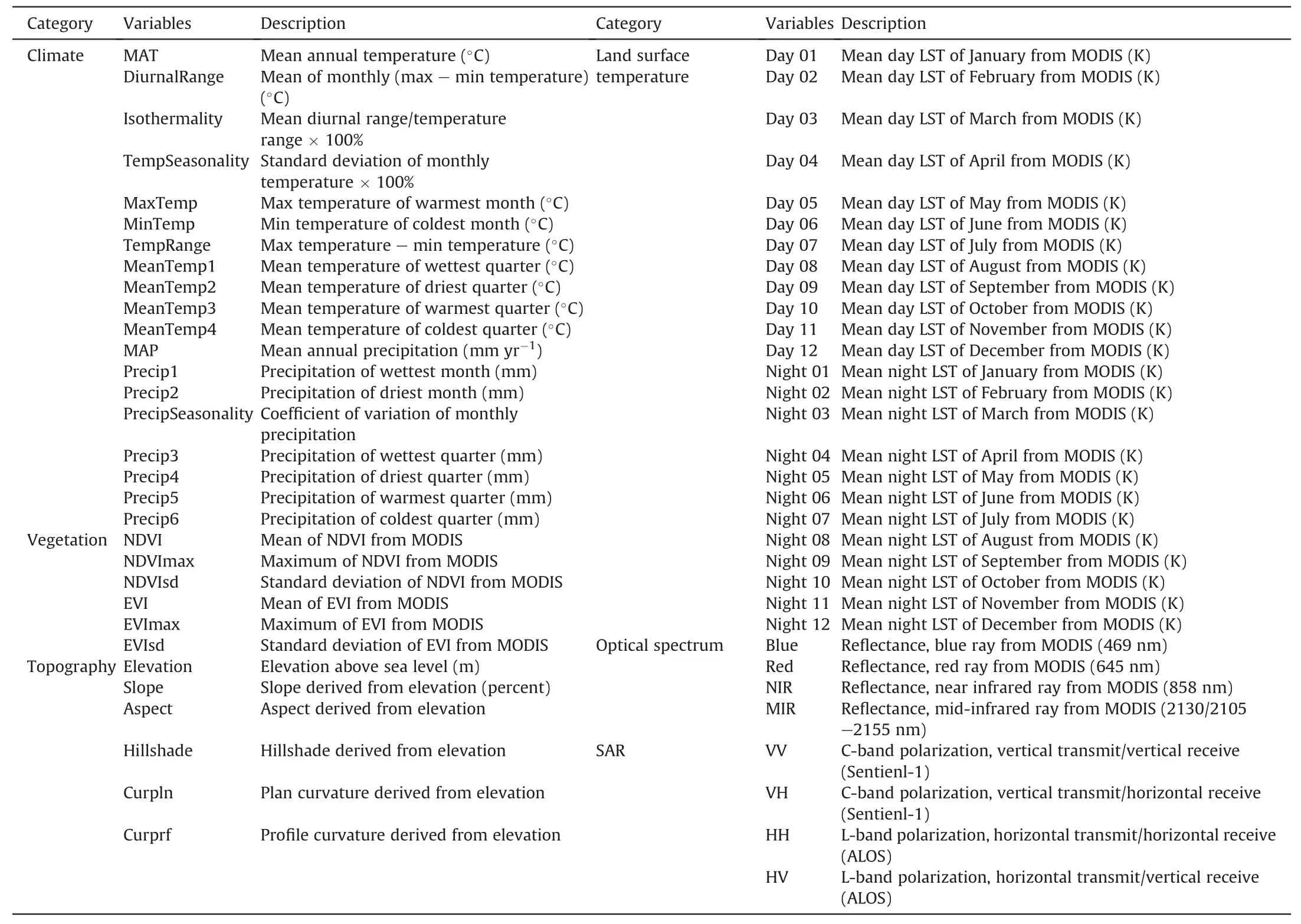
Table 1Environmental variables used for digital mapping.

Machine learning algorithms have also been used for digital mapping.One such machine learning algorithm,random forest(RF),is a robust regression tool in which numerous forecast trees are constructed with a subset of randomly chosen predictors at each node(Breiman,2001).This strategy is stable and against overfitting problem,and prediction is little affected by noise in the training data(Breiman,2001).Additionally,it is user friendly,as only a limited number of parameters need to be tuned and the predictions are generally not very sensitive to the parameters tuning(Liaw&Wiener,2002).Given that remote sensor data have high dimensionality and multi-collinearity,the use of the RF model has been effective in selecting important variables(Genuer et al.,2010).RF has been successfully used as a digital model to map soil organic matter(Yang et al.,2016),texture(Liu,Zhang,et al.,2020),color(Liu,Rossiter,et al.,2020),predict parent material(Heung et al.,2014),and the depth to bedrock(Shangguan et al.,2017).TheKfactor is related to soil properties like organic matter and texture.Since these soil properties have already been predicted successfully,the machine learning algorithm is expected to map theKfactor directly.However,this approach has not yet been evaluated to mapKfactor on a regional scale.

The aims of this study were to(1)examine whether theKfactor can by mapped using RF regression with limited sampling data,and(2)select the important environmental variables served as model inputs for predicting theKfactor.

2.Methods

2.1.Study area

The study is located in the southeast of China.It extends from 24 to 32°N and 116 to 122°E(Fig.1).This 260,564 km2area accounts for a tenth of the Chinese population and almost one fifth of the national GDP,and includes a wide diversity of climate,relief,soil and vegetation.It includes four major landform zones extending from north to south:the alluvial delta plain,hill region,mountain region,and coastal hilly region.Elevation varies from around 0 up to 2100 m above sea level.The climate is subtropical humid,with annual mean temperature(MAT)9.7—18.1°C,and annual mean precipitation(MAP)1500—2170 mm yr-1(Fig.A.1).The majority of the rain falls between April to November,with an average of 25—40 erosive rainfall days in which daily precipitation is greater than or equal to 12 mm(Li et al.,2014).Geologically,the study area consists mainly of alluvium,littoral sediment,light-colored crystalline rock,clastic sedimentary rock and meta-sedimentary rock.According to World Reference Base,the major soil types are Rhodic Ferric Acrisols,Xanthic Ferric Acrisols,Rhodic Ferralsols,Hydragric Anthrosols and Dystric Skeletic Regosols(Shi et al.,2010).Land use in the study area is highly intensive,including long-history farmlands,densely-constructed urban lands,and vast areas of woods,gardens and orchards.The water-induced soil erosion exhibits great spatial variation due to the varied environmental conditions.

2.2.Collection of soil samples

Field sampling for the training dataset was conducted in July of 2019.Because the variation of theKfactor is highly related to soil properties,samples were collected based on soil types in countylevel regions.One to two typical soil genera of the largest area in each county were extracted based on a 1:1,000,000 soil type map(Shi et al.,2004),and the center of each genus was determined as the preliminary sampling point.The specific location of some points was adjusted according to actual field considerations such as accessibility.A total of 101 sampling points was ultimately determined and 0—20 cm surface soils were collected from sampling sites(Fig.1).At each site,three to five augers were taken and fully mixed to obtain a 500 g surface soil sample.Soil samples were airdried and sieved to 2-mm for all analyses.Soil organic matter(SOM)was analyzed via the Walkley-Black wet combustion method(Nelson & Sommers,1983).The volume percentage of clay(＜0.002 mm),silt(0.002—0.05 mm),sand(0.05—2 mm)and very fine sand(0.05—0.1 mm)were determined used a laser diffraction particle size analyzer(LS230,Beckman Coulter).

In this study,theKfactor was estimated from intrinsic soil properties via the nomograph equation(Fig.A.2,Wischmeier &Smith,1978),for the sake of keeping the same calculationmethod as the first-ever nationwide water resources survey in China.As regards the deviation of empirical equations,the nomograph estimations had a larger determination coefficient compared to other equations(such as EPIC and Dg),which were evaluated by natural runoff plot data in eastern China(Zhang et al.,2008).The nomograph equation comprises five variables:the silt plus very fine sand content,the clay content,SOM,the structure coefficient,and the permeability class.Structure coefficients are calculated according to geometric mean diameter of soil aggregates(GMD)and range from 1(diameter＜1 mm)to 4(diameter＞10 mm)(Fieller & Flenley,1992).Permeability classes range from 1(rapid)to 6(very slow)based on soil texture(O'Geen,2013).Finally,theKfactor from the surface horizon(0—20 cm)at the sampling sites was calculated by the nomograph equation as follows.

Fig.1.Study area with soil sampling sites.

where N1represents silt plus very fine sand content(0.002—0.1 mm,%),N2represents clay content(＜0.002 mm,%),OM represent organic matter content(%),S is structure coefficient,and P is permeability class.In this paper,the international system of units(SI)was used for theKfactor.TheKfactor can be converted from the SI metric unit of t·ha·h/(MJ·mm·ha)into the US customary units of ton·ac·h/(100·ac·ft·ton·in)by multiplying with a factor of 7.593.Given the length ofKfactor unit,it was omitted throughout the text.

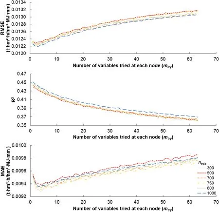
Fig.2.Outputs of 5-fold cross validation vs.number of predictors tried at each node in different numerous trees(ntree).

2.3.Environmental variables

Six categories with 63 environmental variables were selected in this study.Firstly,climate,vegetation and topography were chosen by looking at previous studies,where they are important soil forming factors at a regional scale(McBratney et al.,2003).Additionally,land surface reflectance signals including LST,optical spectrum and radar observations were chosen as predictors of theKfactor.Geological map was not included as predictor,due to its extreme coarse resolution in this study area.

A total of 19 bioclimatic variables were obtained in the WorldClim database(https://www.worldclim.org/data/worldclim21.html)from the year 1970—2000 at 30 arc-second(equal nominal 1 km2)resolution(Fick & Hijmans,2017).Vegetation indexes including Normalized Difference Vegetation Index(NDVI)and Enhanced Vegetation Index(EVI)represent overall status(mean),seasonality(standard deviation)and the best condition(the maximum)of plant growth from August 2000 to July 2020.These were obtained from the MODIS 16-day L3 product at 250 m resolution(Didan,2015),as part of the European Space Agency(ESA)data observations.Elevation was derived from 90 m SRTM DEM(Farr et al.,2007)and five secondary terrain variables(slope,aspect,hillshade,plan curvature and profile curvature)were computed in ArcGIS 10.3.

The ESA's MODIS product was used to derive LST by day and night with 1 km resolution(Wan et al.,2015),using the monthly means from August 2017 to July 2019.The dataset of the MODIS 16-day L3 product also yielded red,blue,near infrared ray(NIR)and mid-infrared ray(MIR)bands with 250 m resolution(Didan,2015),where the average values were calculated from August 2017 to July 2019.Additionally,means of SAR bands were obtained from Sentinel-1 with 10 m resolution(Torres et al.,2012)from August 2017 to July 2019,and ALOS with 25 m resolution(Shimada et al.,2014)from 2007 to 2017 years.Those satellites were launched by ESA and Japan Aerospace Exploration Agency separately.

Except for variables from the WorldClim database,all the environmental variables were downloaded from the Google Earth Engine.The input data have multiple resolutions from 10 m to 1 km.The various environmental variables effect theKfactor on different scales.Climate impacts soils on a large scale(～1 km),vegetation affects soils on a medium scale(250 m),and terrain and radar influence soils on a small scale(10—90 m).The influences of environmental variables are overlaid rather than averaged.The basic unit of digital soil mapping is the pixel.Applying the model to predict theKfactor pixel by pixel requires a uniform spatial resolution of all environmental variables.As a result,the variables were resampled to 250 m resolution inR(http://www.r-project.org/)via bilinear interpolation.The detailed code used for downloading environmental variables and resampling is available on GitHub(https://github.com/ztian37/RF-for-K-factor.git).All environmental variables had been listed in Table 1.

2.4.Random forest regression

The RF model is an ensemble of regression trees where each tree is trained on a bootstrap sample of the training data,and prediction is made by averaging prediction outputs(Breiman,2001).The predicted regression model was built in therandomForestandrangerpackages ofRstatistical software(Liaw & Wiener,2002;Wright & Ziegler,2015).A detailed code for the random forest regression and digital mapping is available on GitHub(https://github.com/ztian37/RF-for-K-factor.git).

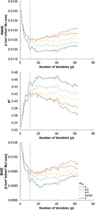
Fig.3.Mean values of 5-fold cross validation with the least important variables removed at each step using different mtry functions(p;p/2;p/4;p1/2;and 2).

2.4.1.Optimization parameters

The split size of the variable subset(mtry)has been chosen from the entire variable set from 1 top,wherepis the total number of variables.The numerous trees of RF regression(ntree)that are grown from bootstrap samples of the entire sample population makes the RF model insensitive to over-fitting.In this study,mtryandntreeare the hyperparameters of RF that tuned to optimize the model.The bestmtrywas chosen fromp,p/2,p/4,p1/2,and 2.To cover the default number and empirical results of the optimalntree,the range ofntreewas set from 300 to 1000.

Two methods were performed for assessing predictions made by different models.Firstly,around 37%of remaining samples from the training dataset were calculated as out-of-bag(OOB)errors.Secondly,models were evaluated through 5-fold cross validation.Since an unbiased estimate of the true prediction error from OOB is not suitable for the case where the number of variables is much greater than the number of subjects,cross validation can reduce the remaining bias(Matthew,2011).Model performance was evaluated by root-mean squared error(RMSE),coefficient of determination(R2),and mean absolute error(MAE)as equations(2)—(4).Among them RMSE measures the closeness of the predictions to the actual values,R2represents the proportion of variation in the sample data that is explained by the model,and MAE shows whether the predictions are on average biased.

wherenis the total number of points in validation,^Yiis the value estimated by the model,Yiis the value observed fromKfactor map,andYiis the average value observed fromKfactor map.

2.4.2.Variable importance

The importance of variables was evaluated to select the most important predictors.We calculated the important scores of increase in mean square error(%IncMSE)in RF regression.The %IncMSE of a given predictoriis calculated as the relative increase in the mean square error(MSE)of the OOB samples which is induced that predictoriis subjected to random permutation while other predictors remain unchanged(Strobl et al.,2008).As a result,the smaller %IncMSE value is,the less important predictoriis.

whereMSEOOBis the MSE of OOB samples,andMSEiOOBis the MSE of OOB samples when given predictoriis permuted.

2.4.3.Variable reduction

The importance score(%IncMSE)of RF is used for predictor reduction.Variable reduction processes adopted from Svetnik et al.(2003)were implemented in this study as follows:

(1)Train a model on all variables and partition the data for 100 replications of 5-fold cross validation.

(2)Use the importance score(%IncMSE)to rank the predictor variables.Record the cross validation test set prediction.

(3)Use the variable ranking to remove the least important variable and retain the model,predicting the cross validation test set.

(4)Compute the RMSE,R2and MAE at each step of removing.

(5)Replicate step(1)—(4)until only one variable remained.

The cases ofmtryequalingp(Bagging),p/2,p/4,p1/2as defaults,and the tuning resultmtry=2 was considered.

2.4.4.Prediction uncertainty

To estimate the uncertainty ofKfactor predictions,we computed the lower and upper limits of a 90% prediction interval via usingrfintervalpackage of R with the OOB method(Zhang et al.,2020).The uncertainty ofKfactor predictions is defined as follows:

whereKupperandKlowerare the upper and lower limit of 90% prediction interval,and^Kis theKvalue estimated by the model.

The prediction interval coverage probability(PICP)for theKfactor was also calculated to evaluate the uncertainty estimation,based on the 101 soil samples with 5-fold cross validation and 100 replications.PICP is the proportion of observations which are enclosed by the corresponding prediction interval(Solomatine &Shrestha,2009).

2.5.Digital mapping

The selective model of RF was applied to scale to the regional area,by extracting the environmental variables values at each grid cell as predictors.The grid maps of theKfactor were displayed in ArcGIS 10.3 using the Albers Equal-area projection.Although climate and LST affect theKfactor on a large spatial scale(～1 km),the resolution of 250 m was chosen for the prediction grid as the important environmental predictors have moderate to high resolutions(10 m—250 m).

3.Results and discussion

3.1.Range and variability of K factors and associated soil properties

Table 2 show the summary statistics of the 101 soil samples.The range of theKfactor was 0.0047—0.0789,and the median value was smaller than the mean value.In the training dataset,theKfactor had a bimodal distribution,with a major peak at 0.037 and a minor peak at 0.064(Fig.A.3).Both SOM and soil texture had a rightskewed distribution,with means and standard deviations of 24.3±16.4 g/kg(SOM),17.5±6.9%(clay),54.8±16.2%(silt),27.7±18.9%(sand)and 6.6±3.0%(very fine sand).

Table A.1Summary of soil erodibility(K factor)mapping methods.

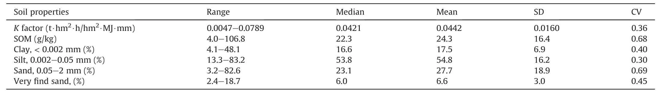
Table 2Summary statistics of soil sampling properties in the study area.

Pearson correlations betweenKfactor and soil properties for the soil samples were-0.412(SOM),0.074(clay),0.800(silt),-0.715(sand),and 0.834(very fine sand).The results show thatKfactor was negatively correlated with SOM and sand content,but positively correlated with clay,silt,and vey find sand.The greater the SOM,the lower theKfactor.SOM is thought to increase wet aggregate stability and therefore enhance erosion resistance of soil(Chenu et al.,2000).TheKfactor was strongly correlated with silt,sand and very fine sand,but less correlated with clay,which corresponds with previous studies(Bonilla & Johnson,2012;Ferreira et al.,2015).This is because clay particles give cohesiveness to soils and are not easily detached and transported by water flow,unlike silt and very fine sand which are susceptible to erosion.Conversely,although sand grains lack of cohesion,they are relatively resistant to erosion because of the particle mass(Young,1980).

3.2.Model performance

3.2.1.Tuning parameters

Fig.2 displays the evaluation outputs for tuning parameters of RF model.Themtrywas tuned from 1 to 63.Overall,RMSE and MAE were increasing and R2was decreasing with increasedmtry.However,the differences between their minimum and maximum values were minor:less than 0.001 for RMSE,0.09 for R2,and 0.0006 for MAE(Fig.2).The results showed that RMSE and MAE reached the minimum values whenmtryranged from 2 to 4,and R2reached the maximum value whenmtrywas 1.When number of trees tuned from 300 to 1000,the differences amongntreesetting were also trivial:less than 0.0001 of RMSE and MAE,and less than 0.008 of R2.

Considering computational efficiency,mtry=2 andntree=500 were chosen in the following study.Themtrywas set small because when there are many relevant predictor variables,not only the strongest influential variables but also the less influential variables should be chosen in the splits(Probst et al.,2019).Additionally,system running time was reducing with decreasingmtryfitted with a polynomial curve(Fig.A.4),which is in agreement with previous results that using a lowmtryvalue and fewer trees result in better runtime efficiency(Wright & Ziegler,2015).There is a threshold where increasingntreewould bring no significant performance gain,but increase the computational cost(Oshiro et al.,2012).It is possible to improve the RF's performance by tuning parameters or reducing variables(Huang & Boutros,2016;Scornet,2017).The most common recommendation is to setntreeto 500 or 1000,andmtrytoorp/3(Belgiu&Drˇagut¸,2016;Probst et al.,2019).In this study,mtryandntreewere tuned by comparing the prediction performance of accuracy values using cross validation,and the outcomes of 5-fold cross validation were not highly varied with the changing ofntreeandmtry.This performance indicates that the parameters tuning bias is negligible in this study.

3.2.2.Variable reduction

Fig.3 shows the model performance with 5-fold cross validation when using the strategy of non-recursive elimination of variables.Overall,the outcomes of cross validation had fairly consistent patterns whenmtry=p,p/2,p/4,p1/2,and 2,where RMSE and MAE were slightly decreasing and R2were increasing as the number of variables reduced top=10(Fig.3).It is worth mentioning that RF models with less than 10 variables had substantially smaller R2,larger RMSE and MAE values and show instabilities,and RF performance with more than 10 variables was relatively similar to that of the full set model(p=63),especially whenmtry=2(Fig.3).A previous study also found that RF modeling is robust to the inclusion of less influential variables(Fox et al.,2017).In this study,a large set of predictors(p=63)might have noisy variables,howeverreducing too many variables(p＜10)in the model will result in instabilities of spatial predictions(Fig.3).The results among full and reduced models indicate that RF is insensitive to the presence of irrelevant predictors.This finding corroborates the variable reduction performance reported by Heung et al.(2014)and Svetnik et al.(2003).For modeling performance,the effects of over-fitting can be eliminated by averaging the predictions of numerous trees(Genuer et al.,2010),thus a full model with 63 variables was chosen for digital mapping.

Fig.4.Variable importance plot based on increase of mean square error(%IncMSE)in random forest(RF)model.See Table 1 for the description of predictor variables.

In general,the best predicted RF model after tuning parameters accounted for less than 48%of the observed variance.An unexplained variability of theKfactor can be due to the reasons such as:(1)the limited sampling data cannot reflect all the environmental conditions of the study area,and those 101 training soil samples were spatially sparse and ignored the subtle variation in small scale;(2)the error of using 250m×250m rastercellsto comparewithsampling points;(3)the deviation caused by the atmosphere correction algorithm(Fick&Hijmans,2017)and geometric calibration for DEM(Farr et al.,2007);(4)the uncertainty of predictedKfactors as function of variant soil properties(Parysow et al.,2003);and(5)seasonalKvalues are highly varied during a year(Mutchler&Carter,1983).To reduce the uncertainty,multiple measurements of soil properties within one year may improveKfactor's predictive accuracy.

3.2.3.Variable importance

Fig.4 ranks the 30 most important variables(other variables having very small importance)based on%IncMSE in RF.The bigger the %IncMSE value,the more important the variable.Two relief parameters,slope and elevation,were identified as the most important predictors.Climate variables such as maximum precipitation and temperature seasonality were also important.It appeared that seasonal changes of climate were more important than the annual mean.In particular,the LST during winter and summer season were more important than that of spring and autumn.The MIR parameter from MODIS was also important.Finally,vegetation indexes particularly NDVI had a relatively high importance.The quantification of the variable importance shed some light into the black box of RF to understand the mechanisms contributing to theKfactor,which is related to intrinsic soil properties and extrinsic erosive forces.

First,theKfactor can be altered by the fine materials migration.In this case,the translocation is closely related to topography(Ibrahim,2018;Zhu et al.,2019),indicating the relief indexes such as slope and elevation should not only be considered to cause soil erosion but also partially mirror soil erodibility(Fig.4).Second,theKfactor is associated with subtle variations in soil water condition(Bryan,2000),as reflected by the fact that precipitation parameters were important variables in this study(Fig.4).However,the direct use of SAR data had poor importance for mapping theKfactor.This might be due to the interference of vegetation cover.Moran et al.(2000)propose that multi-temporal SAR and optical/SAR fusion should be considered for mapping soil moisture.Thus,further study is needed to increase the ability of SAR to predict theKfactor.Additionally,theKfactor is associated with weathering of clay minerals(Khoirullah& Sophian,2019;Shaw et al.,2002).Weathering is to a large extent simulated by warm and humid climates,as reflected by the importance of air temperature and LST here(Fig.4).Lastly,highKfactors are associated with low SOM(Liu et al.,2019).Our study found NDVI and EVI influenced theKfactor by their ability to reflect the provision of SOM(Fig.4).Despite a large set of environmental variables(p=63)used for prediction,half of theKfactor variances were not explained by the RF model.That might be because additional environmental variables were needed to fully capture the variability inK.The relationship between theKfactor and environment conditions is highly complicated.The RF model was only a simplification of these relationships.For example,some environmental variables are dependent on others,and the interaction between predictors is not well explained by the RF approach.The performance of environmental variables needs be further investigated.

3.3.Digital mapping of the K factor

3.3.1.The K factor map

Fig.5c shows the digital map of theKfactor,where the full set model(p=63)withmtry=2 andntree=500 was built.The map of theKfactor was drawn at 250 m resolution,which is because the variables contributed most to predicting theKfactor were slope and elevation with fine resolutions(90 m),and vegetation was also important predictor(250 m).Although climate variables have a coarse resolution(～1 km),the relief and vegetation made a major contribution to the prediction.The predictedKfactor values had the same order of magnitude(0.0431±0.0079)as the existingKfactor map(0.0285±0.0067)provided by the first-ever nationwide water resources survey(Liang et al.,2013).The deviation for predictingKfactor in this approach need further validation by collecting runoff plots data in our study area.

The spatial distribution of theKfactor derived from soil sampling,kriging interpolation and RF prediction followed a similar pattern,where theKfactor is high in the north but low in the middle and south of the study area(Fig.5).The highestKfactor occurred in alluvial delta plain(K=0.065),while the lowest was in the south coastal hilly region(K=0.032).A previous study found that agricultural activities result in a highKvalue(Mancino et al.,2016).This is consistent with our observation that the alluvial delta plain region had highKfactors.A largeKvalue indicates a susceptibility to erosion.However,due to the small slope of plain,the actual soil erosion in the alluvial delta plain is not severe.The forest and orchard in the hilly landform had a less erodible soil,which related to its high sand content and less silt content(Fig.A.5).Vegetation cover of forest and orchard results in a permeable soil surface,and the sand surface is due to the downward movement of fine silt materials into the soil(Chen et al.,2009).Additionally,the dense tree cover results in development of root systems,which contributes to the formation of water-stable aggregates(Erktan et al.,2016).

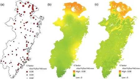
Fig.5.Spatial distribution of soil erodibility(K factor)at study area with(a)101 soil samplings;(b)kriging interpolation;and(c)random forest(RF)model.

The RF model allowed a more detailed prediction ofKfactor than the kriging interpolation method(Fig.5).There are remarkable differences in the level of spatial detail between them.Soil erosion is influenced or can be identified by environmental variables including the soil forming factors(climate,relief,vegetation)and land surface conditions(thermal variation and spectral features)(Fig.4).Digital soil mapping has the ability to produce exhaustive information over a large area by integrating massive amounts of environmental data in a spatial grid,whereas geo-statistical interpolation is only calculated from a limited set of point observations and has smooth changes between these samples.The restricted number of soil samples comprising the training data also limits the model application.The soil samplings represent the major range of conditions occurring in the study area(elevation from 2 to 808 m,NDVI from 0.2 to 0.7,MAT from 13 to 21°C and MAP from 952 to 1841 mm).Although this,we recognized that some extreme environmental conditions may not be covered by the training samples.For these environments not covered,the constructed model in this study may not be effective or get relatively large prediction errors.Besides,the long-distance between samples may not capture the subtle spatial differences of theKfactor.Overall,the soil data limitation would be a drawback of applying the RF model.

3.3.2.Prediction uncertainty

Fig.6 displays the uncertainties in RF predictions ofKfactor,using lower and upper prediction limits at a 90% prediction interval.The 95% prediction interval had a similar spatial pattern with 90%,however the lower prediction limit sometimes had negative values when a 95%interval was used.The lower and upper prediction limits estimated by the RF had similar patterns with mean predictions.Relatively high erodibility soil was in the plain,and low erodibility soil was in the hilly region especially in south coast of study area(Fig.6a and b).The mean predicted K factor in the study area was 0.0431±0.0079 with a bimodal distribution,which was similar to the samples statistics,while the lower limit range was 0.0166±0.0085,and the upper limit was 0.0705±0.0091.In addition,predictions uncertainty appeared to be inversely related to the magnitude of theKfactor.The largest uncertainties were in hilly region especially near south coast,and the smallest uncertainties were in the north plain(Fig.6c).The large uncertainty is probably due to the spatial heterogeneity ofKfactor in hilly areas,for which the sparse sampling was not sufficient to capture these relatively large difference.As a frontline problem of digital mapping,analysis of uncertainty is highly necessary to evaluate accuracy and precision of the spatial information(Liu,Zhang,et al.,2020;Malone et al.,2011).Limit estimation in the study area provides a baseline reference for theKfactor.In addition,prediction interval coverage probability for theKfactor was calculated based on the 101 soil samples with 5-fold cross validation.Under a 90% prediction interval,87% of observations were expected to fall within the lower and upper prediction limits,suggesting that these prediction limits and uncertainty estimated by the RF method were reliable.

3.3.3.Spatial details of map

Fig.7 shows comparison ofKfactor maps at three landscapes.Our predictedKfactor map capture more distinct differences in spatial details,compared to the polygonalKfactor map provided by the nationwide water resources survey(Liang et al.,2013).The polygonalKfactor map has average area of 6.8 km2,while the predictedKfactor map by RF model were at 250 m resolution.The latter one provided much more detailed soil spatial variance,especially for those large heterogeneous regions.This was especially evident in mixed landform regions.RF was effective in extracting the heterogeneity of theKfactor in diverse landforms,such as plain,hill,mountain and coast.For the predicted map,the Taihu basin shows the highKfactors in the plain,contrasting with the lowKfactors of the hill and mountain;the Songgu plain shows the medianKfactors in the plain and lowKfactors in the surrounding upland;the Fuzhou coast shows the pattern of medianKfactors in the plain and lowKfactors in the coastal mountains(Fig.7).

By using the true color image of landscape from Google Earth as a reference,we compared the predictedKfactor map with the polygonal map.Besides the clear regional pattern,there are substantial details within the predicted map.The ground features are more distinct from our prediction than the polygonal map.Differences between the polygonal map and this study are mainly due to their map-making method:polygons from the soil survey data represent an aggregation of the soil-environmental conditions(geology,pedology,landscape,natural boundaries,relief,etc.)in a certain soil type(Heuvelink & Bierkens,1992),whereas every grid cell derived from RF model represents the unique environmental condition which affect theKfactor.The predicted maps at 250 m resolution here are equivalent to the polygon mapping at 1:100,000(1×1 pixel per grid cell)to 1:2,500,000(2×2 pixels per grid cell)scale(Hengl,2006).Additionally,they can show the regional variation in theKfactor as well as details for variations with an extent of 25 hectares(Hengl,2006),which is similar to our study area.Consequently,our predictions better represented spatial variation of theKfactor in study area than the existing map.

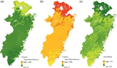
Fig.6.Spatial distribution of random forest(RF)predicted soil erodibility(K factor)at study area with(a)lower limit,(b)upper limit of a 90%prediction interval and(c)uncertainty.

Fig.7.Spatial details of traditional polygonal map,predicted soil erodibility(K factor)map and true color image of(a)—(c)Taihu basin,(d)—(f)Songgu plain,and(g)—(i)Fuzhou coast.

4.Conclusions

This study demonstrated that performing RF regression on environmental variables was an effective approach for mapping theKfactor with limited samples on a regional scale.The model of theKfactor was firstly established from a combination of freely available environmental variables,such as climate dataset and remote sensing images.The predictedKfactor map at 250 m resolution well represents the spatial variation of theKfactor,and clearly shows substantial details in different landforms.This study also provided credible uncertainty maps as a baseline for evaluation.In addition,we found parameter tuning and variable reduction may not necessarily result in a significant improvement in machine learning performance with respect to the cross validation outputs.This research shows that digital soil mapping workflow can successful provide a consistent,detailed view of theKfactor,which was much more precise than existing polygonal map.

The important predictors forKfactor in this study were relief(slope,elevation),climate(max precipitation,temperature seasonality),LST(in winter and summer months),and vegetation(NDVI),while predictors from radar and optical spectra contributed less to the predictions.Seasonal variations of climate were more important than its yearly mean for predicting theKfactor.As a whole,environmental variables interact in a complex way to influence soil properties and thus result in variation of theKfactor.Considering that theKfactor is an important indicator for soil quality assessment and ecological construction,our predictive approach forKfactor mapping is a valuable addition to demonstrate the local heterogeneity of soil erosion risks.Additionally,the identified important predictors can be used as input to models of soil erodibility.

Data availability

All the code used to generateKfactor predictions at southeast China is fully documented via GitHub at https://github.com/ztian37/RF-for-K-factor.git.Digital maps of theKfactor have been archived on Figshare,whereKfactor with random forest model is available at https://doi.org/10.6084/m9.figshare.14245736;Kfactor lower limit is available at: https://doi.org/10.6084/m9.figshare.14245751;Kfactor upper limit is available at:https://doi.org/10.6084/m9.figshare.14245754;andKfactor uncertainty is available at:https://doi.org/10.6084/m9.figshare.14245775.

Declaration of competing interest

The authors declare that they have no known competing financial interests or personal relationships that could have appeared to influence the work reported in this paper.

Acknowledgements

This work was supported by the Jiangsu Grants to Postdoctoral Researchers(2020Z348);the Research Fund from Taihu Basin Authority of Ministry of Water Resources,China(SY-ST-2019-013).The authors gratefully acknowledge the editor and two anonymous reviewers for valuable comments and insightful suggestions.We thanks Dr.Patricia Ann Lazicki for comments on manuscript and polishing the language,and students in University of Chinese Academy of Sciences for involving soil sampling in this study.

Appendices

Fig.A.1.Spatial distribution of(a)elevation,(b)NVDI,(c)MAP and(d)MAT at study area with 101 soil samples.

Fig.A.2.The soil erodibility(K factor)nomograph(Wischmeier & Smith,1978).

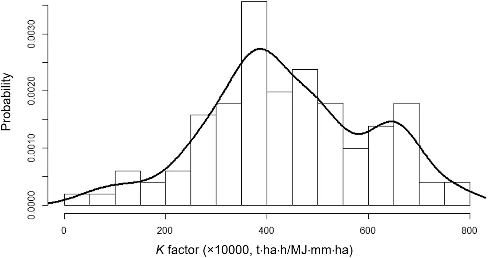
Fig.A.3.Histogram of soil erodibility(K factor)with 101 soil samples..

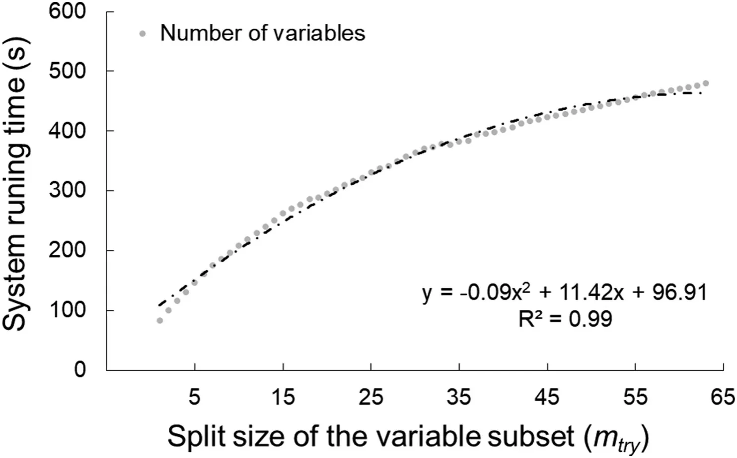
Fig.A.4.System running time of R code using different mtry functions.

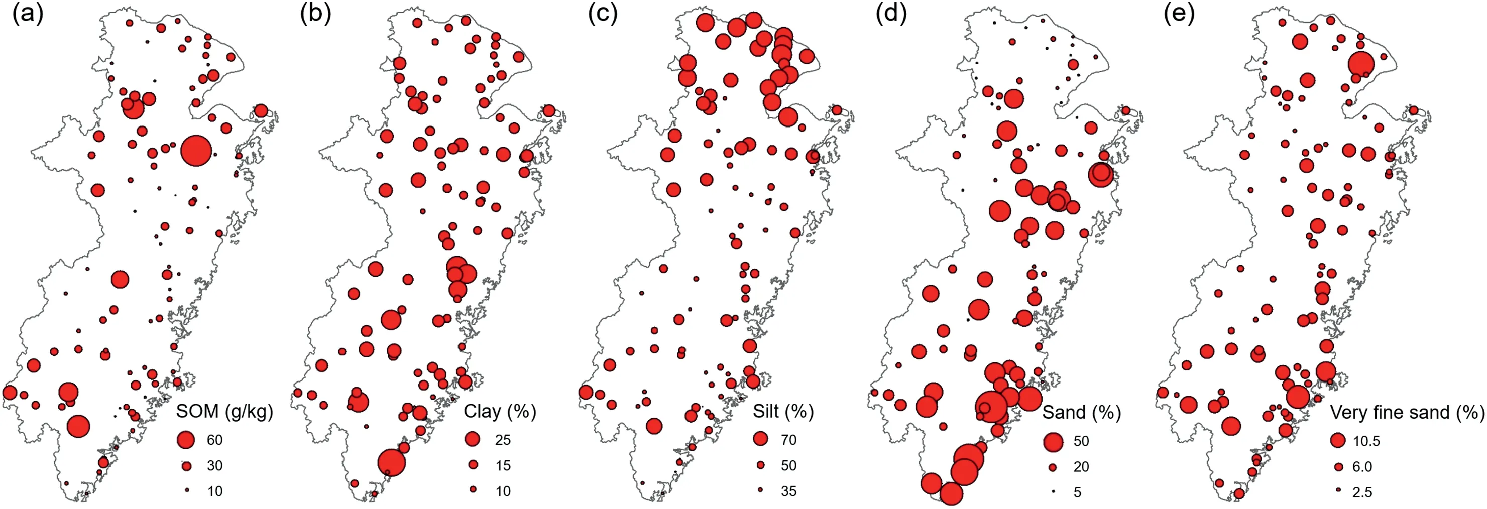
Fig.A.5.Spatial distribution of(a)SOM,(b)clay,(c)silt,(d)sand and(e)very fine sand at study area with 101 soil samples.