An updated isoerodent map of the conterminous United States

Ryan P.MGh ,Dnnis C.Flanagan ,Punt Srivastava ,Brnar A.Engl ,Chi-Hua Huang ,Mark A.Naring

a Purdue University,Agricultural and Biological Engineering,225 South University Street,West Lafayette,IN,47907,USA

b United States Department of Agriculture-Agricultural Research Service,National Soil Erosion Research Laboratory,275 S Russell St,West Lafayette,IN,47907,USA

c University of Maryland,Agricultural Experiment Station,Symons Hall,7998 Regents Drive,College Park,MD,20742-3131,USA

d Purdue University,Agricultural Administration Building,615 West State Street,West Lafayette,IN,47907-2053,USA

e United States Department of Agriculture-Agricultural Research Service,Southwest Watershed Research Center,2000 E Allen Rd,Tucson,AZ,85719,USA

Keywords:Erosion index Erosivity United States USLE RUSLE2 Soil loss

A B S T R A C T:Maps of erosivity,which are also commonly referred to as isoerodent maps,have played a critical role in soil conservation efforts in the United States and around the world.Currently available erosivity maps for the United States are either outdated,conflict with erosivity benchmarking studies,or utilized less advanced spatial mapping methods.Furthermore,it is possible that the same underlying issues with US maps are impacting global maps as well.In this study,we used more than 3400 15-min,fixed-interval precipitation gauges to update the isoerodent map of the conterminous United States.Erosivity values were interpolated using universal kriging under several spatial model configurations and resolutions.The optimal spatial model was selected based on which result had the lowest sample variogram error.Rainfall,erosivity,and erosivity density maps were compared to existing products.Some average annual and annual erosivity results were compared to high-quality erosivity benchmarking publications.Erosivity values from both RUSLE2 and Panagos et al.(2017)were generally lower in the eastern United States and mixed in the western United States compared to our results.Topographic effects resulted in much greater erosivity differences in this study as compared to prior maps.Benchmark comparisons revealed that erosivity maps from this study and others were lower than the benchmark by 14%or more(up to 38%).These findings suggest current practices of storm omission and intensity dampening correction need to be revisited,especially in locations with relatively low-to-moderate rainfall erosivity such as the Midwest or Northeast United States,for example.

Introduction

Rainfall erosivity(R)is one of only two driving factors in USLE,RUSLE,and RUSLE2 erosion prediction models.The other driving factor is soil erodibility(K).These two factors along with four additional modifying factors(L,S,C,and P)comprise the six variables of the Universal Soil Loss Equation(USLE)(Wischmeier,1959).Subsequent modifications of the USLE led to the Revised Universal Soil Loss Equation(RUSLE)model versions 1 and 2(Renard et al.,1997;United States Department of Agriculture-Agricultural Research Service(USDA-ARS),2008).In order to apply each of these models,USLE,RUSLE,or RUSLE2,a user must either calculate their own erosivity inputs or utilize the standard databases or isoerodent maps for these models which are documented in Wischmeier and Smith(1965,1978),Renard et al.(1997),and USDA-ARS(2008),respectively.

Erosivity background

Rainfall erosivity is an empirical measure of rainfall's capacity to cause erosion,and it is defined in USLE as the product of a storm's total kinetic energy and the maximum 30-min intensity of that storm.Wischmeier and Smith(1958)were the first to propose this mathematical relationship and found that it correlated highly(R2＞0.9)to erosion on cultivated and uncultivated plots(Wischmeier,1959).McGehee et al.(n.d.)reviewed essential historical,conceptual,and practical topics of rainfall erosivity applications,which included identifying common obstacles to achieving accurate and reproducible erosivity calculations from diverse precipitation inputs and erosivity mapping discrepancies in literature.Some general steps towards solutions were outlined in that review chapter which is currently in production and is expected to be available in early 2022.However,this manuscript is intended to be a first step towards a potential resolution.We first outline the specific obstacles and present why we consider them obstacles and then list the objectives of this study.

Discrepancies in literature

Since at least 1980,there have been discrepancies reported in isoerodent map values as well as values obtained directly from gauge data(McGregor and Mutchler,1976;McGregor et al.,1980).McGregor et al.(1995)found that both the USLE and RUSLE erosivity values were about 30%too low in northern Mississippi.To arrive at these conclusions,McGregor et al.(1995)used 29 gauges in a small watershed which were of the highest quality—pluviometer or‘breakpoint’gauges.Some progress has been made since then.RUSLE2 documentation provides details about an erosivity database update that resulted in about a 10%increase in values over USLE and RUSLE values(USDA-ARS,2008).However,this still falls short of the findings of McGregor et al.(1995)in northern Mississippi by 1000 to 1500 MJ mm ha-1h-1yr-1(or about 15%—23%)even after accounting for storm omission and energy equation differences.McGehee and Srivastava(2018)confirmed the findings of McGregor et al.(1995)and presented an erosivity map of the southeastern United States which was based on more commonly available 15-min,fixed-interval data.This map was within only a few percent of McGregor et al.(1995)results and consistently higher than erosivity values in USLE,RUSLE,and RUSLE2 maps(Wischmeier&Smith,1965;Renard et al.,1997;USDA-ARS,2008).

It is not just USLE,RUSLE,and RUSLE2 databases that have been published with isoerodent map values significantly lower than the named benchmarking studies.Panagos et al.(2017)published a global erosivity map which was roughly aligned with RUSLE2 database values for the United States.At first,this was puzzling because Panagos et al.(2017)used 5-min,fixed-interval gauges for the United States,which according to Hollinger et al.,2002 and Flanagan et al.(2020)should result in greater erosivity values than those from 15-min,fixed-interval data.However,upon closer investigation of the Panagos et al.(2017)methods,it was found that the study relied upon the Rainfall Intensity Summarization Tool(RIST)(Dabney & Vance,2019)to obtain erosivity estimates.RIST has recently been found to have a subtle bug resulting in significant suppression of erosivity calculations in versions released earlier than May 2019(McGehee et al.,2020);the bug was corrected in May 2019 and RIST now produces similar,though not identical,erosivity estimates to another automated erosivity calculation software,which was used for calculations in this study.McGehee et al.(n.d.)pointed out that prior versions of RIST may be responsible for the lower estimates from Panagos et al.(2017)which were lower than three other global estimates(Nachtergaele et al,2010,2011;Naipal et al.,2015;Yang et al.,2003)as presented in Fig.4 of Panagos et al.(2017).Despite these more prominent examples of conflicting erosivity estimations from the literature,there has been progress towards resolving these mapping discrepancies in the United States.

Recent progress towards resolution

This manuscript represents the culmination of several prior works beginning with the foundational work published by McGregor et al.(1980,1995)to quantify the discrepancy in the existing erosivity maps of the time.Hollinger et al.,(2002)identified some limitations of switching from breakpoint gauges,which were used to develop the original erosivity theory,to fixed-interval gauges,which were(and still are)used to develop isoerodent maps.It seems that some issues may have been resolved in the RUSLE2 erosivity database(USDA-ARS 2008;2013).However,we were unable to find documentation on what specific changes were made to move erosivity values towards more expected values observed with breakpoint gauges.McGehee and Srivastava(2018)showed that 15-min,fixed interval precipitation data could be used to achieve average annual erosivity values very close to those from McGregor et al.(1995)when major differences driven by the type of gauge(e.g.,fixed-interval gauges versus breakpoint gauges)were accounted for.Still,this study was limited to only the southeastern United States and did not account for all differences outlined in McGehee et al.(n.d.),which may account for some annual differences that cancel out in average annual analyses.Flanagan et al.(2020)quantified the impact of fixed-interval gauge limits on precipitation characteristics,erosivity,and physical erosion model predictions.McGehee et al.(n.d.)synthesized all this information in a review that demonstrates the problems,points out the most common obstacles,and suggests proper solution(s)or workarounds for each issue.

Objectives

This manuscript presents the progress to-date by updating the national erosivity map in a way that more rigorously adheres to the principles of the original erosivity relationship discovered and developed by Wischmeier and Smith(1958,1965,1978)and addresses common application obstacles reviewed by McGehee et al.(n.d.).Improving the spatial interpolation model and filling temporal gaps driven by data quality issues are primary focuses in this work.Issues which remain unaddressed in this study are discussed as appropriate.

Methods

Many of the methods employed in this study were first demonstrated in McGehee and Srivastava(2018).That study used 15-min,fixed-interval precipitation data to more closely approximate erosivity from breakpoint data in the southeastern United States.Breakpoint precipitation data preserves measured precipitation characteristics such as intensity to within the precision limits of the gauge.This kind of precipitation data was used to develop the original erosivity relationship and is therefore the most appropriate benchmark for erosivity comparisons.Fixed-interval gauge data are more widespread,but the fixed intervals distort measured precipitation characteristics and introduce error into erosivity calculations.This study builds on the success of the preceding study and incorporates new and superior methods(e.g.,more sophisticated gap-filling and spatial modeling,in particular),which were necessary to obtain a similarly reliable national isoerodent map.A summary of all relevant methods follows.

Study area selection

The conterminous United States was selected as the study area for two reasons.First,isoerodent mapping efforts for USLE,RUSLE,and RUSLE2 used the same area(Wischmeier & Smith,1978;Renard et al.,1997;and USDA-ARS,2008);therefore,comparisons to those studies should use the same analytical bounds.Second,aside from this study's immediate comparison objectives,the United States is home to some of the longest record,most dense,and highest temporal resolution precipitation gauging networks in the world.These datasets will serve important roles in planned future research activities.

Data sources and preprocessing

There were four data sources used in an original capacity within this study.Each dataset,source information,and relevant provideror user-processing information are provided below.

The first and most important dataset used in this study was the National Oceanic and Atmospheric Administration(NOAA)National Center for Environmental Information(NCEI)DSI-3260 15-min land-based precipitation gauge network—the same 15-min data used for erosivity calculations in RUSLE2(USDA-ARS,2008;2013).This dataset can be downloaded through NOAA's National Climatic Data Center(NCDC)web services and is available in the original tape format or in provider-processed datafiles.For this study,the same preprocessing conventions detailed in McGehee and Srivastava(2018)were used to prepare the dataset for erosivity calculations.The most important components of preprocessing include the handling of missing and accumulated data flags.It should also be noted that limitations of that procedure related to‘g’flags,which unreliably report whether a station is operational(Hollinger et al.,2002;McGehee & Srivastava,2018),were addressed through new methods applied in this study,which are related to gap detection and gap-filling(discussed below).Data from more than 3400 stations were downloaded and preprocessed following these conventions for the period from 1970 to 2013.This period reflects the maximum record length of the DSI-3260 dataset before it was modernized again in 2014.Data from 2014 to the present are available in a different format and for different stations which will be incorporated in subsequent research projects.

The analyses of McGehee and Srivastava(2018)were limited to the southeastern United States,so snowfall was not much of a concern in that analysis.In more western and northern regions,snowfall could become a more significant factor in erosion.The way USLE-based models represent snowfall impacts on erosion is by the creation of an equivalent R(Req).This study did not attempt to generate Reqand only aimed to address the question of rainfall erosivity.Therefore,it was important to ensure that snowfall was not accidently included in the rainfall measures from the DSI-3260 gauge data.Per DSI-3260 documentation,gauges likely to see snowfall had snow shields installed at gauges,so there were virtually no snowfall data included in this dataset(though it was possible for some to get past snow shields or to occur where no shields were installed).In those cases after 1996,the provider used a‘Z’flag to indicate that frozen precipitation was likely included in a gauge total.Over time,stations with Z flags present would have snow shields installed.Daily gauge totals with that flag present were removed,but given that Z flags were rare in the dataset,this had insignificant effects on the national erosivity mapping analysis.

Three additional datasets were important for the spatial kriging model and include the Precipitation-elevation Regressions on Independent Slopes Model(PRISM)annual precipitation normal for 1981—2010(Daly et al.,1994),Global Multi-resolution Terrain Elevation Data 2010(GMTED 2010)elevation(Danielson & Gesch,2011),and the NOAA National Ocean Service(NOAA-NOS)distance to nearest coast(Stumpf et al.,2009).The role each of these datasets played in the spatial kriging model are discussed in detail later.

Data quality and screening

Station quality varied significantly in the DSI-3260 dataset.While there are numerous ways to report on data quality,this manuscript focused on two metrics and reported a third metric that may be of potential interest in the future.These metrics include missing and deleted data periods and accumulated depths—all of which can be calculated from data quality flags accompanying the DSI-3260 data(McGehee & Srivastava,2018).Missing and accumulated rainfall data could easily exceed 50% of the total rainfall amount for any given station,which would render even the most capable gap-filling methods unreliable.Therefore,stations were screened to reduce the strain put on the gap-filling procedure(described below).Deleted period percentages were reported because they reflect provider processing impacts on each station,though they may not be of immediate use to users.It was rare to find stations with high deleted percentages,especially after station screening;thus,this metric was not used in a significant role in this study.Fig.1 shows ordinary kriging maps of these metadata metrics for all available stations before screening,and it provides important insight into how unscreened stations or narrowly sufficient stations may impact the following analyses as a whole or influence problematic regions.

Stations were screened by a minimum record length(10 years),a maximum accumulated depth percentage(20%),and a maximum missing period percentage(20%).The screening options and screening outcomes for this study were reported and compared to a similar study in the southeastern United States in Table 1.As can be seen in Table 1,this study has a less strict screening method than was employed by McGehee and Srivastava(2018).That study did not utilize a sophisticated gap-filling method like this one,which necessitated the more sophisticated screening method(i.e.,the minimum months per year condition).The screening method used by McGehee and Srivastava(2018)would prove to be too restrictive in locations with consistently missing dry months or winter months in arid and northern climates,respectively.The screening method used in this study should be considered an improvement over the preceding study when paired with the more sophisticated gap-filling approach.

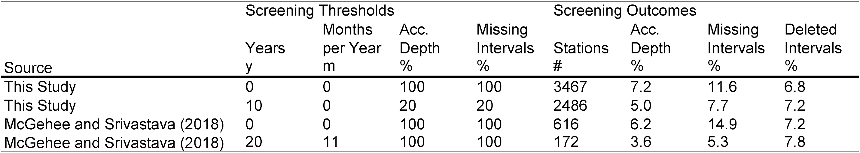
Table 1Station screening thresholds and outcomes compared between this study and a similar preceding study(McGehee and Srivastava,2018).See the accompanying in-text description for screening details and importance.Accumulation is abbreviated acc.below.

Gap detection and gap-filling

Given the unavoidable reality of missing and accumulated data in the DSI-3260 precipitation dataset,a critical component to any workflow involving this data is gap detection and gap-filling.Three gap-filling options were compared in this study including:no gapfilling,linear metadata-informed adjustments,and multiple imputation by chained equations(MICE)based gap-filling(van Buuren & Groothuis-Oudshoorn,2011).Only the MICE-filled option actually resulted in completely filled time series based on the input interval data.There are many possible MICE configurations for gap-filling objectives,and the one used in this study was identical to the default configuration utilized by the WEPP Climate File Formatter(WEPPCLIFF)v1.5(McGehee et al.,2020).

Since the MICE-based gap-filling model is stochastic,several iterations were executed to determine the variability of this filling option.The average erosivity for the screened stations which satisfied the WEPPCLIFF gap-filling model's minimum requirements varied on the order of tens of metric erosivity units(or ones of the English equivalents),which is quite insignificant for much of the conterminous United States.Therefore,only one random run was used for the mapping exercise to reduce the computational demand and data storage requirement for this study.

Fig.1.Ordinary kriging maps of DSI-3260 station metadata(1970—2013)for(a)and(d)accumulated precipitation(as a percent of total measured depth);(b)and(e)missing periods(as a percent of total observation period);and(c)and(f)deleted periods(as a percent of total observation period);for pre-screened stations at 32 km(a—c)and 1 km(d—f)resolution.

Erosivity calculations

Erosivity was computed using the energy equation prescribed in RUSLE2 documentation(USDA-ARS,2008;2013),which was a modified and more accurate(Nearing et al.,2017)version of the equation presented in Brown and Foster(1987).Storms were separated by breaks defined as less than 1.27 mm of rainfall in 6 h,which was identical to previous erosivity literature(Wischmeier&Smith,1965,1978;Renard et al.,1997).These calculations were performed using WEPPCLIFF(McGehee et al.,2020).Storms less than 12.7 mm in total depth were optionally removed unless the 15-min intensity was greater than 24.13 mm h-1.In other words,two sets of maps were produced—one with all storms and one with these storms omitted,similar to RUSLE2 conventions).Snowfall was excluded from erosivity calculations.Freeze-thaw and snowmelt effects on erosion are represented in RUSLE2 using an equivalent R-factor(Req)where those effects are significant.This study did not attempt to update Reqvalues for snowfall.

Note that this study does not omit storms of return periods greater than 50 years(like RUSLE2)for two reasons.First,determining a 50-year erosivity event using an average record length of only 32 gap-filled years is an unnecessarily uncertain approach,since one cannot reliably determine a 50-year erosivity event.Those 50-year precipitation events could be determined from many other longer and more complete precipitation datasets,but 50-year precipitation events are not equivalent to 50-year erosivity events.Second,no methods were described in the RUSLE2 documentation regarding how these events were removed from its standard climate database,so no comparable analysis could be performed for this study.

Spatial model and resolution

Several spatial kriging model variants were tested for use in the final mapping implementation.Variants included ordinary and universal kriging models utilizing various combinations of spatial variables.Spatial model performance(i.e.,error sum of squares(SSERR)between the sample variogram and the fitted model)was tested at 10 km resolution(a moderate resolution)for six models.The optimal model from the 10 km test was then deployed for all resolutions(1,2,4,8,16,and 32 km)and variables of interest(precipitation,erosivity,and erosivity density).Resolutions were selected based on sequential doubling of the finest PRISM precipitation dataset resolution(800 m)after resampling to 1 km.

Intensity correction

15-min fixed-interval precipitation gauge data were used for erosivity calculations in this study.This kind of data has been widely reported to underestimate or dampen precipitation intensity values,though there is some observed variability in the degree to which this occurs.To account for the underestimation,calculated erosivity values were increased by 4% following conventions from Hollinger et al.,2002,USDA-ARS(2008),and McGehee and Srivastava(2018).An important discussion on intensity correction follows the results section of this manuscript to address this practice in light of recent related research efforts.

External mapping comparisons

Three mapping comparisons were made to external datasets.First,rainfall prediction maps from this study were compared to PRISM precipitation maps from the most comparable time period.This comparison served multiple purposes including:relating total rainfall predicted in this study to that of total precipitation(rainfall plus snowfall)in PRISM;contrasting the impact of(rainfall)storm omission and its interaction with 15-min,fixed-interval gauge data;and laying the foundation for a rainfall validation study in the future.The incorporation of precipitation-based comparisons follows the precedent of McGehee and Srivastava(2018)in pairing erosivity analyses with precipitation analyses.These exercises should help those who wish to compare this work with their own by showing how much rainfall can be associated with the erosivity values provided herein.

Second,erosivity prediction maps from this study were compared to the RUSLE2 erosivity map from its documentation(USDA-ARS,2008)and the more recent erosivity map from Panagos et al.(2017).These comparisons were included based on existing concerns regarding the accuracy of erosivity values used in USLEbased models(McGregor et al.,1995)as well as those obtained using RIST(McGehee et al.,2020).Two comparisons were performed for each map including a comparison of each map's values to those of the original storm omission recommendations from Wischmeier and Smith(1965,1978)and to those of all storms in light of the challenges presented by using fixed-interval precipitation data as opposed to breakpoint precipitation data.All other erosivity calculations followed RUSLE2 documentation conventions(i.e.,the same energy equation and storm separation were used,as mentioned earlier).

For each prediction variable—formally known as predictand—map,there were two options for how to arrive at the final map.Each map could either be obtained directly through the universal kriging procedure,or one map could be derived from the other two.The former approach would result in the best possible map for each variable given the input data and spatial model parameters;however,only the latter would guarantee synonymous maps(i.e.,any two could be used to reproduce the third).Given that presenting all results would be impractical and that the latter approach required an arbitrary(and less transparent)choice of which predictand would be favored for the analysis,the former approach was taken.If predictands(precipitation,erosivity,and erosivity density)could be mapped simultaneously(i.e.,in the same spatial kriging model)to better generalize the overall prediction model across all predictands,this could be revisited in the future and updated.Since that was not feasible in the project's time constraints,prediction maps were provided for each variable,separately.Since a separate spatial model was used for each predictand(Table 2),there are slight differences when comparing derived results from any two predictand maps to the third predictand map,though this should be a relatively small difference corresponding to the error of the given prediction model and resulting maps.

Table 2Spatial kriging model performance comparisons at 10 km resolution based on MICE-filled 15-min gauge data prediction variables—formally known as predictands—(pcp,ei,and ed)and up to five predictor variables(prism,z,cd,y,and x)which are defined below.Lower sum of squares error(SSERR)is better.

Results and discussion

Results were organized into three sections including:temporal gap-filling model and spatial kriging model comparisons,national isoerodent map comparisons,and finally comparisons to existing erosivity studies.Discussion was provided throughout the results where appropriate,and topical discussion on critical points followed the results presentation.

Gap-filling and kriging model comparisons

The impact of the three gap-filling options are shown in Fig.2.It is clear from this figure that station quality had important impacts on national mapping exercises.Both the unfilled and metadataadjusted approaches led to more inconsistent(not smooth)mapping results.The WEPPCLIFF-MICE implementation(van Buuren&Groothuis-Oudshoorn,2011;McGehee et al.,2020)is a purelytemporal gap-filling method,which means that there is no spatial component to this approach,yet it resulted in a very consistent final map.This was achieved without calibration of any parameters,and it demonstrated the potential and accuracy of multivariate gapfilling methods in such applications.Internal tests during this study revealed that storms filled by the WEPPCLIFF-MICE procedure were less erosive than their original counterparts.Therefore,all MICE-based results in this study may be expected to increase in future WEPPCLIFF releases.

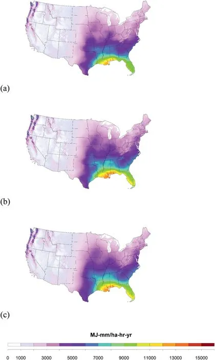
Fig.2.Universal kriging maps of average annual erosivity(1970—2013)for(a)no gapfilling,(b)linear,metadata-based gap-filling,and(c)MICE-based gap-filling for all storms at 1 km resolution.

Spatial kriging performance was influenced by two primary factors:the kriging model and the spatial resolution.The process for selecting the kriging model was discussed earlier in the methods section.Table 2 shows the SSERR for 18 model-variable combinations(6 spatial models x 3 prediction variables).The error sum of squares calculation from Table 2 was a stochastic result requiring many runs for a robust approximation.However,in light of the computational demand of calculating and storing 108 national kriging results(3 variables x 3 gap-filling options x 2 storm inclusion options x 6 spatial resolutions),only one run of these 108 models was used to obtain values presented in Table 2.The 4thorder model was the best model for both erosivity and erosivity density,and the 2ndorder model was best for precipitation.These results make sense because PRISM already accounts for elevation,coastal distance,and latitude(among several others)in its model,which was more comprehensive than the 4thorder model this study employed for precipitation.Erosivity on the other hand is less closely linked to precipitation amount alone and more driven by energy and intensity,which seem to also be related to elevation,coastal distance,and latitude(and probably others not assessed in this study).The same model(4thorder)was used for all prediction variables going forward even though the 2ndorder model for precipitation resulted in moderately lower SSERR in testing.

The other primary factor influencing kriging results was the spatial resolution.The six spatial resolutions are compared in Fig.3.Finer spatial resolutions were generally more important where there was significant change in any important predictor variable(e.g.,elevation or precipitation changes in the West Coast,the Rocky and Appalachian mountain ranges,etc.).However,in addition to the direct impacts,there were also indirect impacts to the selected spatial model itself.For example,since elevation changes were obscured by coarser resolutions,they could not be as easily identified as an important predictor variable when analyzed at the coarser resolutions.For this reason,the finer resolutions did not merely result in more resolving power for the prediction map,but they actually resulted in different predictions.SSERR values for MICE-filled erosivity predictions at 32,16,8,4,2,and 1 km resolutions were 2.06·104,1.65·104,8.09·103,5.83·103,5.37·103,and 5.12·103,respectively.Keep in mind that these were sample variogram errors,and the determination of more robust values was too computationally demanding.Note in Fig.3 how the prediction for the state of Iowa was more erosive with finer resolutions.These dynamic changes(with finer resolutions)were at least partially responsible for the prediction model achieving much lower SSERR by changing the spatial resolution alone.Note how spatial resolution impacted universal kriging results(Fig.3)as compared to ordinary kriging results(Fig.1);higher spatial resolution does not impact ordinary kriging patterns but does impact universal kriging patterns.

Fig.3.Universal kriging maps of MICE-filled average annual erosivity(1970—2013)for all storms at(a)32 km,(b)16 km,(c)8 km,(d)4 km,(e)2 km,and(f)1 km resolution.

In addition to interaction between spatial resolution and the selected prediction model,there was also interaction between spatial resolution and storm omission.Fig.4 shows the impact of storm omission on the prediction map at 32 km and 1 km resolutions.At both spatial resolutions,predictions with smaller storms omitted were lower;however,at the finer(1 km)resolution,these changes were much more significant for some locations than for others.Similar patterns were observed in the other finer resolution maps(e.g.,the 2,4,and 8 km maps)with decreasing significance with coarser resolutions.This phenomenon may have been what prompted comments in Hollinger et al.,2002 and USDA-ARS(2008)regarding observations of spatial inconsistencies in RUSLE and RUSLE2 erosivity maps,respectively.It seems that this issue stems from storm omission rules’interaction with local climate patterns where perhaps similar moisture content is being condensed and precipitated to the ground in characteristically different events due to local topographic(or other)effects.Rigid storm omission rules may then be an infeasible practice if either more accurate or smoother erosivity maps are desired.

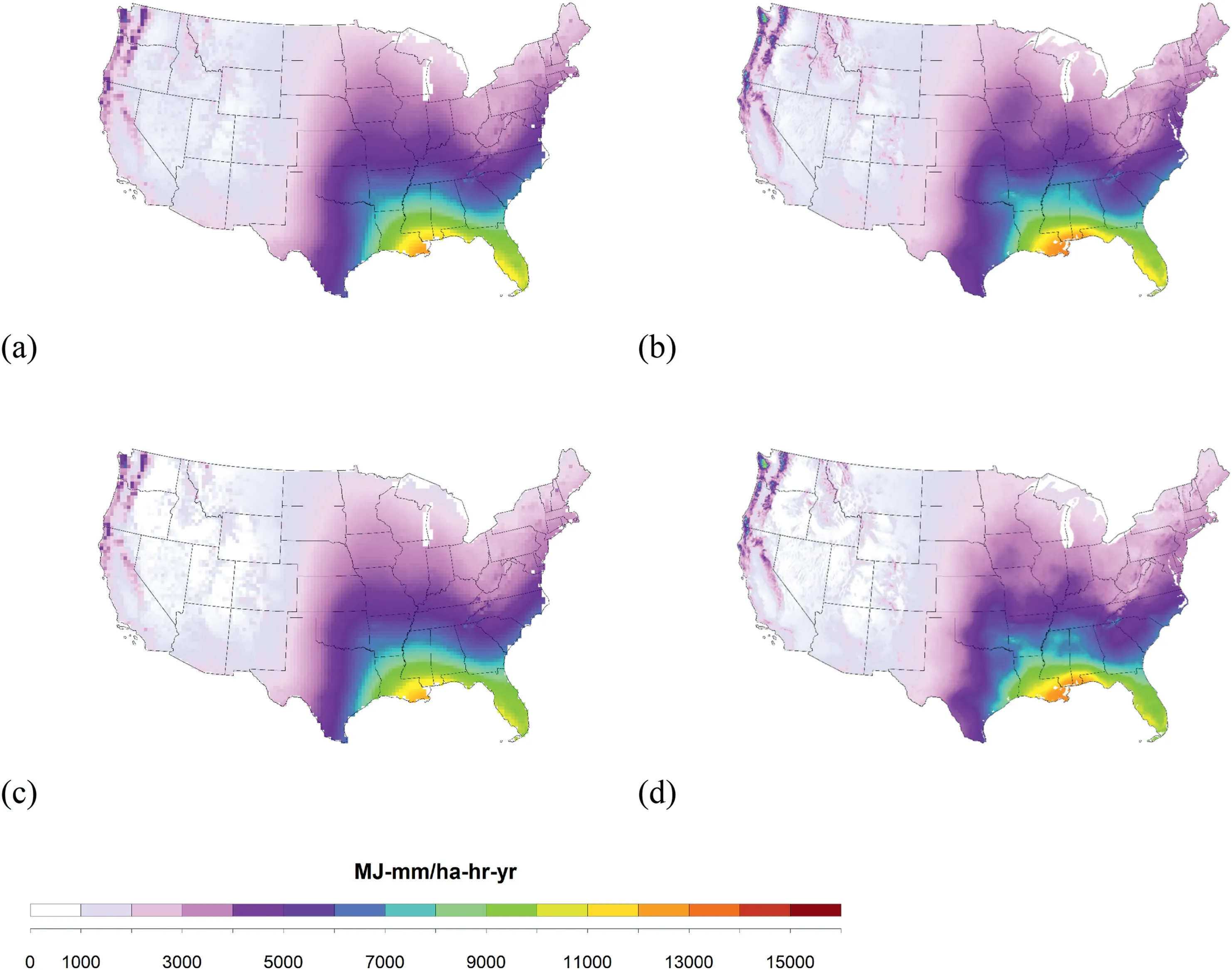
Fig.4.Universal kriging maps of MICE-filled average annual erosivity(1970—2013)for all storms at(a)32 km and(b)1 km resolution and with small,low intensity storms omitted at(c)32 km and(d)1 km resolution.

Irregular contours in the maps with smaller storms omitted were not unique to erosivity predictions alone;they were observed in both rainfall prediction maps(Fig.5)and erosivity density maps(Fig.6),though the impact was much more muted in the erosivity density maps.Note the differences between omitting storms and retaining them in Figs.5 and 6.Fig.5 was included to highlight differences in total precipitation(PRISM),total rainfall(all storms from the 15-min data),and rainfall of‘erosion-causing’storms(retained storms from the 15-min data).This figure should help to understand how much rainfall may be missing from this national analysis in future research efforts.Note,for example,that in the southeastern United States there is little snowfall,but the difference between the interpolated rainfall data with gaps filled and the PRISM precipitation surface is still significant(Fig.5b—c).

Many kinds of precipitation gauges have been known to have problems or recording biases that may need correction,and the DSI-3260 dataset was no exception to this rule.Even though gaps were filled by a sophisticated gap-filling method,it was still possible for the measured data to be biased from the actual amount,and some have documented this amount to be around 5%—10%more or less depending on gauge height,gauge type,and wind conditions onsite(Rodda,1968;Muchan,2016;Rodda & Dixon,2012;Sevruk et al.,2009).Muchan(2016)provided a particularly useful summary of several prior research investigations into these matters.This manuscript did not account for the effect of gage heights and wind conditions on measured rainfall amounts.Nonetheless,this will be investigated and properly accounted for in future publications when the necessary data are available.

Erosivity density prediction maps were generally much smoother than those for rainfall and erosivity,which can be attributed to its lower coefficient of variation(USDA-ARS,2008;McGehee&Srivastava,2018).As expected,the erosivity densities of larger storms(smaller storms excluded)were found to be much larger than the erosivity densities for all storms(Fig.6).These maps showed that while there were some minor exceptions,erosivity density patterns across the United States were similar whether smaller storms were omitted or retained.This was in contrast to precipitation and erosivity,which seemed to be impacted more irregularly by storm omission.

National isoerodent maps

Two national erosivity maps(smaller storms omitted and all storms,respectively)were compared to current maps from RUSLE2 documentation(USDA-ARS,2008)and Panagos et al.(2017)in Fig.7.Maps from this study and RUSLE2 documentation were based on 15-min,fixed-interval data primarily(RUSLE2 documentation did not specify exactly what other datasets may have been used in its creation;however,given that there were only a few options available in that time period it could be surmised that the DSI-3260 data were the primary source for that analysis).The map from Panagos et al.(2017)was based on primarily 5-min rainfall data.Erosivity calculations for all maps were based on the RUSLE2 energy equation and storm separation conventions.Maps from 15-min precipitation gauges had the initially calculated 30-min maximum intensity increased by 4% based on recommendations from Hollinger et al.,2002.Although 4% was recommended by Hollinger et al.,2002,Flanagan et al.(2020)suggested that 4%may not be enough for at least some locations and observed that 9%was more appropriate for a station near Boston,Massachusetts.It seemed that none of these maps were corrected for underestimation of precipitation by the gauges,though that remained a likely source of potential underestimation.This was not corrected in the current study primarily because the information required to do so was not readily available,but that remains a potential place for improvement in future erosivity mapping efforts.The main sources of differences in maps from Fig.7 include the following(for RUSLE2,Panagos et al.(2017),and this study,respectively):different time periods(1960—1999 vs.2006—2016 vs.1970—2013),different gapfilling approaches(no specified gap-filling for either RUSLE2 or Panagos et al.(2017)Maps vs.MICE-filled),storm omission(smaller storms and 50-year or greater storms omitted vs.only smaller storms omitted vs.either small storms omitted or all storms retained),and finally,spatial model(ordinary kriging vs.Gaussian Process Regression vs.universal kriging).

Fig.5.Universal kriging maps of MICE-filled average annual rainfall(a)with smaller storms omitted(1970—2013;excluding snowfall),(b)including all storms(1970—2013;excluding snowfall),and(c)PRISM precipitation(1980—2010;including snowfall),at 1 km resolution.

Absolute and relative difference maps for Fig.7 erosivity maps are shown in Fig.8(for omitted storms)and Fig.9(for all storms).For all difference figures,values above or below the plot range were substituted with the maximum or minimum plot value,respectively.This was done for plotting purposes only.In each of these maps(Figs.8 and 9),it was clear that differences from the spatial models were most significant in the western United States,where topography is known to have a significant impact on precipitation patterns.Since this area also had the lowest precipitation in the United States,the relative differences there were extreme.

Fig.8 shows how the RUSLE2 and Panagos et al.(2017)maps compare to an updated erosivity map based on a nearly identical approach to its original mapping approach(storms were not removed based on any return period and the original Wischmeier and Smith(1978)storm omission recommendation was used).The omission of 50-year and greater return period storms should not have a significant effect on the final maps since those storms would be rare by definition.Furthermore,defining a 50-year storm with only 29 years of data at most(the DSI-3260 gauges were installed in 1970 and RUSLE2 only used data up to 1999)introduces unnecessary uncertainty into any climate analysis.The RUSLE2 storm omission convention was slightly different from the Wischmeier and Smith(1978)definition in that RUSLE2 also omits storms with 15-min intensity greater than 24.13 mm h-1that are still less than 12.7 mm in depth.These storms were uncommon,especially for 15-min gauge data;and therefore,they were also of little significance to this study.

Fig.9 shows how the RUSLE2 and Panagos et al.(2017)maps compare to an updated erosivity map based on including all storms.This comparison undoubtedly included some storms which USLE,RUSLE,and RUSLE2 technology and the original erosivity relationship were not developed to handle,namely,small,low-intensity storms.However,since all these analyses and maps were based on fixed interval precipitation data,this figure also includes storms important to erosivity theory(moderate-or high-intensity storms of small depths)that would have been otherwise removed.This is due to an interaction between erosivity calculation methods and precipitation gauge types,which has now been well-documented(McGregor et al.,1995;Hollinger et al.,2002;McGehee &Srivastava,2018;Flanagan et al.,2020;McGehee et al.,n.d.).Therefore,if one were to adhere to the original erosivity theory more rigorously,accounting for the particular gauge type being used,an updated erosivity map for RUSLE2 would be somewhere between the differences shown in Figs.8 and 9.However,that would still not be accounting for all intensity dampening by the fixed-interval effect(Flanagan et al.,2020)nor for the underestimation of rainfall measurements in gauges installed above ground(Muchan,2016)nor for the precision limitation of the DSI-3260 gauges(2.54 mm as opposed to the modern standard of 0.254 mm),which may interact with all prior effects.

Significant differences in average annual erosivity values were noted in every region of the United States as compared to both RUSLE2 and Panagos et al.(2017)maps.These differences were most significant in the western United States where erosivity values tend to be lower on average,change more drastically due to topographic effects,and where spatial interpolation models vary in their ability to represent those changes.However,even in regions with high or moderate erosivity values and relatively little topographic change,there were significant differences.For example,Fig.10 shows the isoerodent lines and relative differences between this study and RUSLE2 for the state of Iowa and surrounding areas.When excluding smaller storms from erosivity estimates these differences were as high as 38% in the northwestern region of the state where values from the RUSLE2 map were about 2350 MJ mm ha-1hr-1yr-1and values from this study were about 3250 MJ mm ha-1hr-1yr-1.The primary reasons for these differences were discussed earlier,but the relative effect on erosivity values can become much more pronounced in regions with lower erosivity values such as Iowa.These results highlight the need for an erosivity benchmarking study in the Midwest United States—a region where agriculture is the dominant land use,soils tend to be more highly erodible,and where erosivity differences between this study and RUSLE2 were substantial.

Fig.6.Universal kriging maps of MICE-filled average annual erosivity density(1970—2013;excluding snowfall)for(a)with smaller storms omitted and(b)all storms,at 1 km resolution.

Comparison to erosivity benchmarks

McGregor et al.(1995)provided benchmark values for different energy equations and storm omission practices based on breakpoint precipitation data for the years 1982—1992.Table 3 compares these benchmark values(averaged across 29 breakpoint stations)from the Goodwin Creek Watershed,Mississippi(1982—1992)to corresponding values from the nearest precipitation gauge in this study(1970—2013).Comparisons were made between exact years and all years similar to that provided in McGehee and Srivastava(2018)but with the improved methodology of this study.Several points can be made regarding Table 3.

First,even after gap-filling the 15-min data,there was a rainfall deficit of about 5% which was consistent with findings from Muchan(2016)regarding the underestimation of rainfall in common precipitation gauges.Second,erosivity deficits can largely,but not totally,be explained by rainfall deficits(they may also be partially explained by uncorrected intensity dampening effects on kinetic energy estimation).Third,erosivity density comparisons were nearly identical,which were less affected by undermeasured precipitation.Finally,the same patterns were observed as from McGehee and Srivastava(2018)even after gap-filling,which supports the conclusion that the effects of 15-min,fixed-interval data on erosivity calculations were not primarily gap-induced.Years of higher than normal erosivity tended to be underestimated,and years of lower than normal erosivity tended to be overestimated by the fixed-interval data.

A benchmark comparison was also made outside the southeastern United States,which produced very similar findings to those from the Goodwin Creek Watershed(McGregor et al.,1995).Flanagan et al.(2020)used the best quality station from a 1-min,high-precision,fixed-interval weather network just outside of Boston,Massachusetts to determine average annual erosivity there.A novel breakpoint conversion procedure was used with the 1-min data to produce pseudo-breakpoint data,and it was compared to values from this study and to the current RUSLE2 erosivity database.In that comparison,storms smaller than 12.7 mm were omitted(regardless of intensity),and the RUSLE2 energy equation and erosivity ruleset were used to calculate EI.

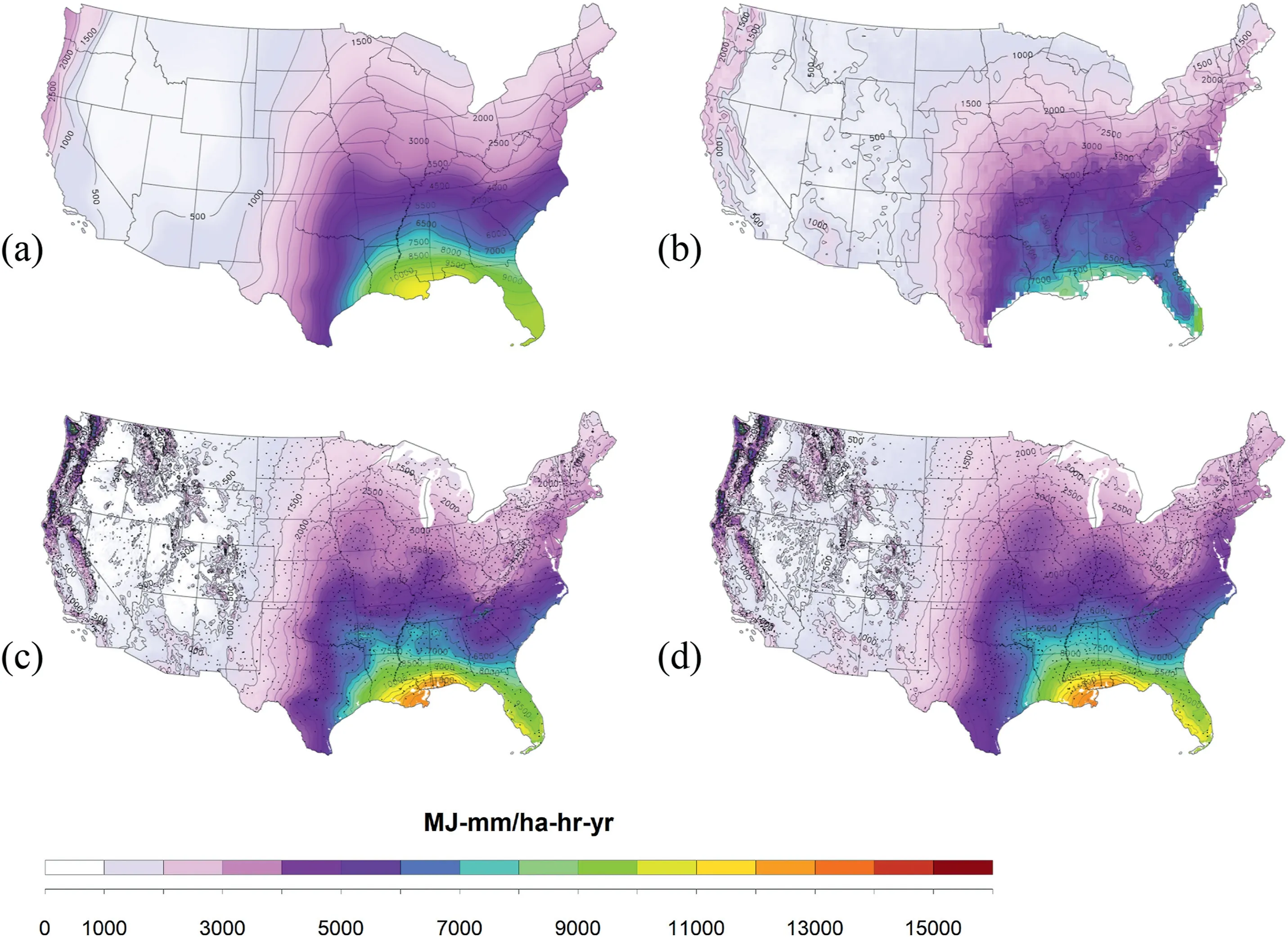
Fig.7.Average annual erosivity maps from(a)the default United States climate database for RUSLE2(1960—1999)(USDA-ARS 2008),(b)Panagos et al.(2017),and from this study(1970—2013)at 1 km resolution with MICE-based gap-filling with(c)smaller storms omitted,and(d)all storms included.

The results of these comparisons are presented in Table 4.As expected,Panagos et al.(2017)erosivity values were the most different from benchmarks likely due to the impact of the RIST software bug in addition to gauge undermeasurement.RUSLE2 erosivity values(USDA-ARS,2008)were the next most different followed by this study with smaller storms omitted and this study with all storms included.The fact that the benchmark studies were evaluated over different time periods than the various prediction maps did not seem to have a significant impact on the results(partially because the time periods overlap significantly and average annual values are less sensitive to variability than annual erosivity or other smaller temporal aggregations).Despite differences in time periods which may cause relatively minor differences in average annual erosivity values,this comparison seems to indicate that current erosivity estimation practices are inadequate to account for differences between breakpoint and fixed-interval precipitation data.Predicted erosivity values from all evaluated studies were between 14% and 38% less than the corresponding benchmark values.McGregor et al.(1995)stated that a difference of about 30% was unacceptable for erosivity estimations.Potential explanations for differences between this study's erosivity estimations and the benchmark values are discussed in the following paragraphs.

Limitations and future work

This study should not be considered a final analysis of erosivity in the United States.In fact,the erosivity values presented in this study are likely to be lower than those in reality due to undermeasured rainfall even after gap-filling(Muchan,2016).This was supported by benchmark comparison results(Table 4)as well as the findings of other previously published works(discussed in detail below).Several remaining issues need to be resolved before a conclusive erosivity mapping study could be conducted and published,and that is in reference to utilizing current 15-min gauges as opposed to forthcoming or next-generation technologies which may present new challenges themselves.For instance,the proper storm omission practice,intensity dampening correction,undermeasuring correction,gap-filling(may have been sufficiently solved in this study),or gauge precision interactions with all prior items remain essentially unaddressed.Some of these items listed above have been explored to a limited degree,but there may not be quite enough evidence to thoroughly settle these issues.A summary of each item is presented in the following text.

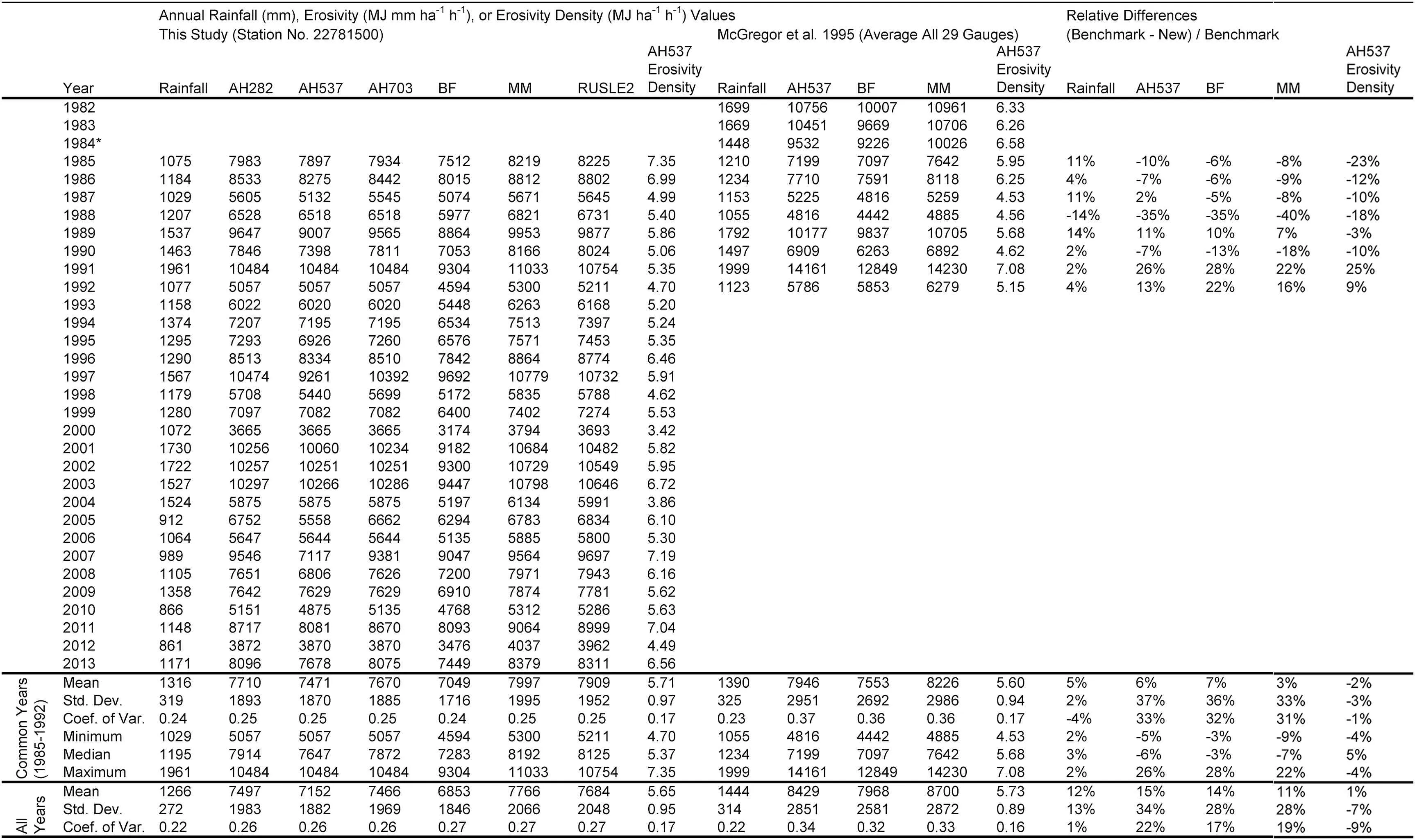
Table 3A comparison of the average of 29 breakpoint gauges(McGregor et al.,1995)and the nearest 15-min,fixed-interval gauge(this study;Station No.22781500)across shared years(1985—1992)and all years for the two studies.*The year 1984 was excluded due to a switch to digital recorders,which impacted data quality in that year.

Table 4A comparison of benchmark average annual erosivity values from McGregor et al.(1995)and Flanagan et al.(2020)to predicted average annual erosivity maps from this study(with and without smaller storms omitted),RUSLE2 documentation(USDA-ARS 2008),and Panagos et al.(2017).Relative differences are computed using the benchmark as the baseline.

Storm omission practices

Storm omission effects were evaluated in this study,but it is important to remember that Wischmeier and Smith(1965,1978)made those recommendations based on breakpoint precipitation gauge data,which is substantially different from fixed-interval data such as that used in this study and in the RUSLE2 climate database.Fixed-interval data,especially coarser intervals such as 10-,15-,and 30-min or longer,dampen breakpoint intensity values,and these effects seem to be more significant in smaller events rather than larger events(Flanagan et al.,2020).This is not to mention that much of the DSI-3260 dataset has a measurement precision of only 2.54 mm(0.1 inch),which makes the storm omission threshold more marginal in some climates and may partly explain why RUSLE2 documentation noted difficulty obtaining consistent spatial results in parts of the United States.Therefore,the combination of smaller depth events,precision limitations,and interval limitations calls into question the validity of storm omission thresholds and practices when using the DSI-3260 or similar datasets for erosivity mapping.Based on findings from McGehee and Srivastava(2018)and Flanagan et al.(2020),storm omission with 15-min,fixed interval data can result in much larger differences in moderate or coarse fixed-interval data than that reported by McGregor et al.(1995)for breakpoint data.McGregor et al.(1995)reported a difference of 3.5% for the Goodwin Creek Watershed;McGehee and Srivastava(2018)reported an average difference of 9% for the Southeast;and this study found that the national average difference was slightly above 10%when omitting storms with total depth less than 12.7 mm.

Fig.8.Average annual erosivity difference maps for absolute differences calculated as this study with smaller storms omitted(Fig.7c)minus either(a)RUSLE2(Fig.7a)or(b)Panagos et al.(2017)(Fig.7b)and relative differences(c)RUSLE2(Fig.8a)or(d)Panagos et al.(2017)(Fig.8b)divided by Fig.7a or 7 b,respectively.Red areas indicate erosivity predictions from this study were higher than the comparison map,and blue areas indicate the opposite.

Intensity dampening correction

Flanagan et al.(2020)evaluated and quantified common fixedinterval precipitation gauge resolution impacts on precipitation intensity,erosivity(an empirical soil loss driver),and WEPP runoff and soil loss predictions.King et al.(2000)performed a similar evaluation for Green-Ampt Mein-Larson infiltration and runoff.The common finding was that coarser,fixed-interval precipitation inputs(10-min or coarser)led to significantly lower precipitation intensity,and this kind of data should be adjusted for the underestimation appropriately.This dampening impacts both kinetic energy estimation and maximum 30-min intensities of storms,but only the latter is accounted for with the 4%increase recommended by Hollinger et al.,2002.Flanagan et al.(2020)suggested that 9%was perhaps a more appropriate correction for intensity dampening in at least the northeastern United States.However,the dampening seems to be influenced by regional storm characteristics themselves,so it may be more appropriate to correct or adjust values by the storm characteristics rather than a constant.

Precipitation undermeasurement correction

Precipitation gauges installed above ground level underestimate or undermeasure rainfall(Rodda,1968;Rodda & Dixon,2012;Sevruk et al.,2009).This is influenced by wind speed at the time of the precipitation event.Muchan(2016)summarized and quantified the effect of gauge height(above ground)and wind speed on precipitation gauge underestimation.DSI-3260 gauges were installed above ground,though obtaining the gauge heights and wind speeds necessary for a precise correction may prove to be too difficult.A more imprecise correction may be necessary for this particular dataset until this information can be found or sufficiently accounted for.

Fig.9.Average annual erosivity difference maps for absolute differences calculated as this study with all storms included(Fig.7d)minus either(a)RUSLE2(Fig.7a)or(b)Panagos et al.(2017)(Fig.7b)and relative differences(c)RUSLE2(Fig.9a)or(d)Panagos et al.(2017)(Fig.9b)divided by Fig.7a or 7 b,respectively.Red areas indicate erosivity predictions from this study were higher than the comparison map,and blue areas indicate the opposite.

Temporal gap-filling

Gap-filling was absolutely necessary for this study.While the erosivity density approach offers some reprieve from this issue,there is still the potential for bias(e.g.,months with missing events,intra-annual climate variability interaction with missing months,and inter-annual climate variability interaction with missing years,etc.).Whether one opts for the standard erosivity approach or the erosivity density approach,an advanced gap-filling method can reduce uncertainty introduced by these unavoidable circumstances.As demonstrated in this study,temporal gap-filling(with no spatial information of any kind provided)resulted in better spatial maps of erosivity than using no gap-filling method or station metadata to adjust measured values(Fig.2).This was also key to enabling more stations to pass screening and achieving more densified observations for more skillful mapping of areas with greater topographic variability.Gap-filling resulted in a national average increase of 14.3% and 11.5% for rainfall and erosivity,respectively,as well as an average decrease of 2.4% for erosivity density.As mentioned before,it appears that the gap-filled storms from WEPPCLIFF are less vigorous(i.e.,lower 30-min maximum intensity)than non-filled storms,which may be addressed in a future update and would result in mild to moderate increases for regions with significant missing or accumulated data.

Gauge precision correction

Finally,an item which has received very little attention is gauge precision.To our knowledge,only McGehee et al.(n.d.)has demonstrated the impact of precision on erosivity calculations,though it has been discussed in McGehee and Srivastava(2018),Flanagan et al.(2020),and probably other works as well.Coarser precision leads to amplified effects of fixed-interval gauges(i.e.,overestimation or underestimation factors experience greater degrees of influence over coarser precision gauges).All data used in this analysis were of the coarser 2.54 mm(0.1 inch)precision,which is more consistent with the RUSLE2 data source since higher resolution data from the 15-min gauges were only available after November 1993.It is foreseeable that a potential adjustment could be developed in the future,but this particular issue has not received enough attention to recommend a generalized correction procedure at this time.

Forthcoming gridded precipitation datasets

Fig.10.Relative difference maps from this study(Figs.8c and 9c)zoomed and centered on the state of Iowa.Overlayed isoerodent lines in blue dashes are RUSLE2 database values(USDA-ARS 2008),while solid black lines are from this study with(a)smaller storms omitted and(b)all storms.Note that the color map interval was halved for this figure(as compared to Figs.8c and 9c).Red areas indicate erosivity predictions from this study were greater,and blue areas indicate the opposite.Units for erosivity are MJ mm ha-1 hr-1 yr-1.

With gridded products of finer temporal and spatial resolution becoming more available and building longer record lengths,those products stand to bolster erosivity studies significantly.When they are ready to be used for erosivity studies,they will inherit all the same temporal uncertainties of gauged networks plus a different form of spatial uncertainty(as compared to gauged networks).The erosion modeling community must be prepared or at least begin preparing for this new and exciting change,which will no doubt bring about new possibilities and potentially more skillful modeling capabilities.This research accelerates the arrival of this future,and,hopefully,contributes to a seamless and simple transition.

Summary and conclusions

An updated erosivity map(isoerodent map)for the conterminous United States was presented which was calculated based on 15-min,fixed-interval data for the years 1970—2013(Fig.7c).This map was created using almost identical rules to existing maps from RUSLE2 documentation and Panagos et al.(2017).Then another erosivity map(Fig.7d)was presented to demonstrate that storm omission practices are causing more storms(and associated erosivity)to be omitted than observed by McGregor et al.(1995)or Wischmeier and Smith(1958,1965,and 1978)from breakpoint precipitation data,which were used to develop the erosivity relationship used in the USLE family of models.Without accounting for rainfall undermeasurement,better intensity dampening correction,gauge precision limitations,or spatial resolution limitations,a more accurate national erosivity estimate based on 15-min,fixed interval data would fall between Fig.7c and d.The most accurate erosivity estimate from this dataset would need to account for each of these issues and shall be addressed systematically in subsequent research efforts.Until each of these issues are addressed,erosivity estimates(including those from this study)are likely to continue to fall below breakpoint-derived(or similar high-resolution product-derived)erosivity benchmarks.For now,Fig.7c—d provide closerapproximations of benchmark erosivities than existing maps from RUSLE2 and Panagos et al.(2017).

Maps from this study were produced using a sophisticated gapfilling model which significantly improved the temporal record of many stations in the study and the spatial consistency of interpolated maps.Standard storm omission and intensity correction methods were used to calculate various erosivity scenarios.Several universal kriging models and spatial resolutions were investigated,with a modestly advanced model and 1 km resolution resulting in the lowest prediction error.Rainfall and erosivity density prediction maps were also produced so that erosivity predictions could be understood in the context of rainfall measurements(or undermeasurements to be more precise).No corrections were applied for intensity dampening of kinetic energy,precipitation gauge undermeasurement,or precision limitations.Erosivity prediction maps were compared to the current RUSLE2(USDA-ARS,2008)and Panagos et al.(2017)erosivity maps,and select locations were compared to peer-reviewed erosivity benchmarks.While maps from this study exhibited greater erosivity in general,all erosivity maps evaluated—those from this study,RUSLE2 documentation,and Panagos et al.(2017)—had erosivity values substantially lower than those determined from higher quality precipitation gauges in Mississippi and Massachusetts.These findings suggested that the current practices for storm omission,intensity correction,gauge undermeasurement correction,and precision correction of 15-min,fixed interval data may all need to be reevaluated with high quality precipitation datasets in the near future.

The original erosivity relationship and erosion plot correlations to erosivity were based on breakpoint precipitation data.Trade-offs in gauge quality and capability were accepted in order to utilize more commonly available and dense precipitation networks such as the DSI-3260 dataset.Applications of these less precise technologies deviated from the original Wischmeier and Smith(1958)erosivity calculation and led to conflicting erosivity databases and maps that could not be readily compared or reproduced.The diversity of precipitation measurement technologies and tools have complicated solutions to common application obstacles,and undocumented variations in handling those unique data streams have hindered efforts to resolve said discrepancies.This manuscript has systematically identified and discussed all of the known potential issues of using coarser,fixed-interval precipitation gauge data in lieu of breakpoint data,and this research has provided a summary of progress-to-date as well as a direction for future research which will be necessary to resolve the published discrepancies in erosivity mapping studies and observed erosivity benchmarks.

Funding

This work was supported with funds from the USDA-Agricultural Research Service National Soil Erosion Research Laboratory through a cooperative project with the Purdue University Department of Agricultural & Biological Engineering.

Declaration of competing interest

None.