Serviceability evaluation of water supply networks under seismic loads utilizing their operational physical mechanism

Miao Huiquan and Li Jie

1. Key Laboratory of Urban Security and Disaster Engineering of China Ministry of Education, Beijing University of Technology, Beijing 100124, China

2. State Key Laboratory of Disaster Reduction in Civil Engineering, Tongji University, Shanghai 200092, China

3. Department of Structural Engineering, Tongji University, Shanghai 200092, China

Abstract: The serviceability of water supply networks (WSNs) under seismic loads has significant importance for estimating the probable losses and the impact of diminished functionality on affected communities. The innovation presented in this paper is suggesting a new strategy to evaluate the seismic serviceability of WSNs, utilizing their operational physical mechanism. On one hand, this method can obtain the seismic serviceability of each node as well as entire WSNs. On the other hand, this method can dynamically reflect the propagation of randomness from ground motions to WSNs. First, a finite element model is established to capture the seismic response of buried pipe networks, and a leakage model is suggested to obtain the leakage area of WSNs. Second, the transient flow analysis of WSNs with or without leakage is derived to obtain dynamic water flow and pressure. Third, the seismic serviceability of WSNs is analyzed based on the probability density evolution method (PDEM). Finally, the seismic serviceability of a real WSN in Mianzhu city is assessed to illustrate the method. The case study shows that randomness from the ground motions can obviously affect the leakage state and the probability density of the nodal head during earthquakes.

Keywords: water supply networks; seismic serviceability; nodal water pressure; stochastic ground motions; probability density evolution method

1 Introduction

Water supply networks (WSNs) are important components of lifeline systems, which include buried pipes, pumps, valves, etc., to deliver water from sources to customers, reservoirs, tanks, and cisterns, etc., to meet the needs of life-sustainance, fire protection, emergency relief, and various other infrastructures. However, a great many previous earthquake investigations have proved that the seismic serviceability of WSNs is still very weak (O'Rourke, 1996; Takada and Hassani,2015; Bouziou and O'Rourke, 2017). Once WSNs are damaged, residential, commercial, and industrial activities can be disrupted for a long time, which will result in severe economic losses, including direct loss to repair damaged parts and indirect loss by shutting down facilities and factories. The most important is that a shortage of water may severely affect firefighting and post-earthquake emergency relief (Ariman and Muleski, 1981). The most infamous example of such factors is probably the 1906 San Francisco earthquake,in which the lack of water was mainly responsible for the great fire and the epidemics that occurred in the aftermath of the earthquake (Ariman and Muleski,1981). Also, seismic serviceability is an important aspect of the resilience of communities (Herreraet al.,2016; Ouyanget al., 2012; Liuet al., 2014). Obviously,a water delivery system does not have solely social and economic influences on communities but also requires technical and organizational considerations (Chang and Shinozuka, 2004). Therefore, the serviceability of WSNs under the influence of earthquakes is crucial for estimating probable losses and the impact of diminished functionality on an affected community.

The seismic serviceability analysis of WSNs has aroused many researchers′ interest. In 1981, Shinozukaet al. first evaluated the serviceability of the WSN in the city of Los Angeles by using the Monte Carlo simulation (MCS) method, in which a point leakage model for the hydraulic equation of WSNs in a daily operational state was used (Shinozukaet al., 1981).Next, the MCS method was further developed by some other researchers. For example, in 1985, O′Rourkeet al.analyzed the seismic serviceability of the WSN in the city of San Francisco (O′Rourkeet al., 1985). In 1998,Hwanget al. performed a hydraulic simulation analysis to assess the serviceability of the WSN in the city of Memphis, with the aid of geographic information system(GIS) technology (Hwanget al., 1998). In 2008, Adachi and Ellingwood suggested a method for analyzing the serviceability of a WSN following an earthquake, which took into account the dependence on water system functionality with regard to the availability of electrical power (Adachi and Ellingwood, 2008). In 2009, they considered the impact of the spatial correlation of seismic intensity on the serviceability of a networked system situated in a region of moderate seismicity (Adachi and Ellingwood, 2009). Although the MCS method can approximate the probability distribution of the reliability index and cope with multiple system-specific modeling and operation conditions, its computational complexity is reflected in exponentially increasing running time as a function of the number of infrastructure component nodes and links (Dueñas-Osorio and Rojo, 2011).

A second popular method is the first-order reliability method (FORM). In 2004, Chen and Li suggested a first-order second-moment (FOSM) method for approximating the reliability of post-earthquake WSNs (Chen and Li, 2004). After introducing a point leakage model to the hydraulic equation of WSNs, the performance of the system can be obtained. The case study showed that the FOSM method was more efficient than the MCS method. Furthermore, in 2015, Liuet al.compared the efficiency and precision of the FOSM method and two first-order third-moment methods (Liuet al., 2015b). The results showed that the two thirdmoment methods presented a higher degree of accuracy than the FOSM method. Generally, the moment method has relatively high computational efficiency, but only portions of probabilistic information, such as the mean,the second-moment, and the third-moment, which can be obtained while the whole probability distribution of the seismic response is out of reach. In addition, when the performance function is complicated or implicit,the utilization of the FOSM method will become much more difficult (Xu and Kong, 2018). Of course, besides the methods mentioned above, there are also some other models for estimating the seismic serviceability of WSNs, such as the probabilistic analytical approach,which is based on graph theory (Li and He, 2002); the fuzzy probabilistic approach, which is based on fuzzy mathematics (Fu and Kapelan, 2011); and methods employed on the basis of the concept of resilience(Ellingwoodet al., 2016; Guidottiet al., 2016), etc. In addition, the performance and serviceability of some special facilities, such as storage tanks as an integral part of the water supply system, have also attracted the attention of many researchers (Brunesiet al., 2015;Bakaliset al., 2017; Merino Velaet al., 2019).

Another noticeable problem is the time-varying characteristics of water supply and water demand when earthquakes happen. “Time” should be important for the seismic serviceability analysis of WSNs. To evaluate the function of damaged WSNs, steady flow theory is often used by many researchers (Shinozukaet al., 1981; Wang and O′Rourke, 2008; Liu,et al., 2015). However, the steady flow theory can only deal with the steady flow itself. Essentially, it implies that water flow in WSNs does not change with time. Obviously, for real WSNs,this method, used to analyze water flow, is very rough.The obtained water head and flow information lacks a description of time, while in a real earthquake both should of these factors should be dynamic. On the other hand, the water demand of different nodes should also change with time. In 1984, Kamedeet al., for the first time, considered the time-varying characteristics of water demand (Kamedaet al., 1984). They supposed that the post-earthquake period for water demand could be divided into four stages, namely, firefighting,drinking, minimum living standard, and full recovery.Liuet al. (2015b) pointed out that the demand flow of a node will decrease after earthquakes. They used a linear equation to amend the demand water head of different nodes of WSNs. This is also a rough description of the effect of time. Therefore, considering the two issues mentioned above, transient flow theory is utilized in this paper to reflect the dynamic change of water flow.“Time” becomes an effective physical quantity in the transient flow model (Chaudhry, 2014). By this means,the time-varying characteristics of water supply and water demand can be effectively reflected.

In 2004, Li and Chen suggested a new method, named the probability density evolution method (PDEM), for analyzing a nonlinear stochastic dynamic system with random parameters, subjected to stochastic excitations(Li and Chen, 2004). PDEM reveals the internal relationships between probability density evolution and physical system state evolution. For one thing, compared to moment methods, it can obtain the probability distribution function (PDF) and the cumulative distribution function (CDF) of a stochastic dynamic system at any moment (Li and Chen, 2009; Li, 2016).For another, compared to the MCS method, it contains relatively high-efficiency calculations, which have been widely used in stochastic seismic response (Liuet al.,2015a), system reliability evolution (Liet al., 2007),and optimal control of structures (Penget al., 2016).In order to assess the dynamic serviceability of WSNs under the influence of earthquakes, a new physicallybased method via use of the PDEM is suggested in this paper. The method is realized by combing the stochastic seismic response of buried pipe networks and transient flow analysis of WSNs with or without leakage. On the one hand, this method is capable of evaluating the dynamic functional reliability of each node in WSNs and global WSNs. Thus, the dynamic seismic serviceability of each node and global WSNs can be obtained. On the other hand, this method can clearly reflect the propagation of randomness from ground motions to WSNs. Accordingly, it can be found that the randomness of ground motions significantly affects the service characteristics of different nodes and whole WSNs. To achieve this purpose, the following three steps are taken.First, a finite element model is established to capture the seismic response of buried pipe networks and a leakage model is suggested to ascertain the leakage area of WSNs subjected to earthquakes. Second, the transient flow of WSNs with or without leakage is derived to obtain dynamic water flow and pressure in WSNs. Third,considering the effects of random ground motions, the dynamic serviceability of WSNs under the influence of earthquakes is analyzed via use of the PDEM.

This paper is organized into seven sections. Following the introduction, section 2 provides a detailed analysis of the physical mechanisms of WSNs to establish a basic framework for damaged WSNs under the influence of earthquakes. Accordingly, section 3 introduces a finite element model to obtain the seismic response of buried pipe networks and a dynamic leakage model during or after earthquakes to identify the leakage area of WSNs.Section 4 presents the transient flow method for single pipes and pipe networks. The characteristic equations for the transient flow in pipe networks with or without leakage are derived. Section 5 focuses on the application of the PDEM to the dynamic serviceability analysis of WSNs under the influence of earthquakes. Meanwhile,the solving steps of the numerical algorithm are presented in detail. In section 6 an actual WSN in Mianzhu is analyzed by the method suggested in this paper as an example. The dynamic water head and serviceability of some nodes, as well as the global reliability of the WSN are presented. Lastly, conclusions are enumerated in section 7.

2 Physical mechanisms of WSNs

2.1 Physical mechanisms of WSNs in normal conditions

To analyze the seismic function of WSNs subjected to earthquakes, the function of WSNs in normal conditions should be analyzed first. The physical mechanisms of WSNs are illustrated by Fig. 1.

Fig. 1 Physical mechanisms of WSNs in normal conditions

An actual WSN normally includes three parts. The first is water sources, such as water towers, reservoirs,pumps, etc. The second is pipe networks, which include straight pipes, tee pipes, elbow pipes, valves, and other complicated fittings. For simplicity, only pipes are considered in this paper because the number of pipes is much larger than that of valves. The third part includes different customers, including communities, hospitals,factories, etc. The needs of customers are mainly the requirement of water head and flow, as well as water quality at different nodes of the networks.

Different indexes can be used to evaluate the serviceability of different nodes of water supply networks, such as nodal water flow, water pressure,and water quality. When the flow rate is used as the index, the presence or absence of water is a relatively intuitive phenomenon, but for ordinary consumers or stakeholders the amount of water flow to meet the needs of those nodes is not easy to understand. This indicator is abstract. Specifically, different water heads represent the water demand for persons living on different floors.For example, when a water head is 10, 16, or 22 m, it means that the water can be transported to the 3rd, 5th,and 7th floors without assistance from other equipment.Therefore, this index is easy to understand and intuitive for consumers and related managers. In general, after nodal pressure is determined, the nodal flow information is ascertained. Taking this into consideration, the nodal head is selected as the serviceability index for this paper.This index is also popular among other researchers (e.g.,Gheisiet al., 2016). Water quality is a more stringent indicator. At this time, “water” becomes a mixture of many substances rather than a single commodity(Ostfeld, 2004). The authors expect that this index can be studied in future work.

The steady-state or transient flow theory can be utilized to model water flow in WSNs. The difference between them lies in whether they consider the inertial force of water. The former neglects the inertial force of water, which essentially supposes that water pressure and flow in the network do not change over time(Cunha and Sousa, 1999). However, the latter considers the inertial force of water. As a result, it can reflect a dynamic change of water flow in WSNs caused by some disturbances, such as power outages or adjustments to valves and pumps (Karney and McInnis, 1992).Therefore, the steady-state flow theory neglects the description of “time” while the transient flow theory can account for it. In addition, modern WSNs are more complicated than traditional ones. Transient flow is common and can produce accurate results. Therefore,the transient flow theory is a more appropriate method for designing and analyzing modern WSNs (Karney and McInnis, 1992). This article focuses on the dynamic seismic serviceability of WSNs. “Time” is a key factor used to describe the system. Therefore, transient flow theory is used to model dynamic water flow in WSNs.

2.2 Physical mechanisms of WSNs under the influence of earthquakes

When earthquakes occur, WSNs may be damaged by seismic loads. Traditionally, a pipe network is an object for independent research. However, for a functional analysis of WSNs subjected to earthquakes, the earthquake, the site to bury the pipe network, the pipe network, and the water flow all constitute a composite system. A separate analysis of certain parts is one-sided.The physical mechanisms of WSNs under the influence of earthquakes must be studied systematically. For instance, the research framework proposed in this article is an open framework. Other elements of the water supply system, such as water towers and storage tanks,can all be taken into consideration to make the model more comprehensive and accurate.

The physical mechanisms of WSNs under the influence of earthquakes can be divided into four parts,as illustrated in Fig. 2. In Part 1, a normal WSN works as in the analysis included in section 2.1. In Part 2,when an earthquake takes place, a seismic field will impose itself on a pipe network. Unlike water towers or high-rise buildings, the inertial force of underground pipelines can be neglected. When an earthquake occurs,due to the propagation of seismic waves, the site where the underground pipelines are buried will also vibrate,thereby driving the movement of the pipelines. Common pipelines include segmented and continuous ones. In this paper, only the destruction of segmented pipelines is considered. Segmented pipelines are generally formed by pipe segments with different lengths and different types of joints (ALA, 2005). For segmented pipelines,the deformation of the ground is mainly absorbed by the joints of the pipelines. This is mainly because the stiffness of the joints is small relative to the stiffness of the pipe body (Liuet al., 2018). When an earthquake is severe, the movement of the ground will cause the joints to move in axial and rotational directions and crack the filling materials of joints. As a result, the joints will be damaged. In Part 3 it is noted that leakage appears in the damaged joints. Water flow in the WSN will change and the nodal water head will vary with time. In Part 4,considering the demand water head of different nodes,the function of different nodes and the global WSN will change.

Fig. 2 Physical mechanisms of WSNs under the influence of earthquakes

Therefore, to evaluate the serviceability of a damaged WSN, three steps must be implemented.The first is to build a finite element model to capture the stochastic behaviors of buried pipe networks. The second step is to obtain the rate of dynamic water flow in the damaged WSN. Herein, the equations of transient flow in the network is solved by employing the method of characteristics (Chaudhry, 2014). The third step considers the demand water head of different nodes, by which the serviceability of those nodes can be estimated.In addition, if the weighting factors of different nodes can be ensured, the serviceability of the global WSN also can be obtained. Of course, a random earthquake field model also is needed to produce acceleration samples (Wang and Li, 2012). By means of the PDEM,the stochastic behaviors of buried pipes can be obtained(Liuet al., 2015b). In this paper, the PDEM is utilized to further study the dynamic water flow of the WSN and evaluate the seismic serviceability of the WSN subjected to random ground motions.

3 Seismic response of buried pipe networks

3.1 Seismic behaviors of buried pipe networks

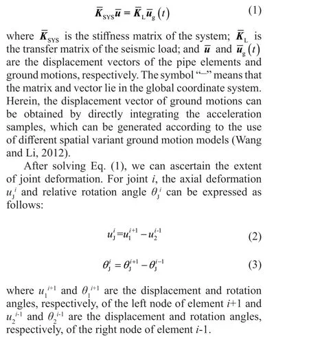
To identify the seismic behaviors of buried pipe networks, a finite element model (Liuet al., 2015a) is adopted in this paper. Considering that the inertial force of underground pipelines subjected to the seismic load can be ignored, this model is a quasi-static model. In this method, the motion equations of the pipe network can be expressed as:

3.2 Leakage model of pipe networks

To determine the relationship between leakage flow and water pressure, the following point leakage model is used (Chen and Li, 2004):

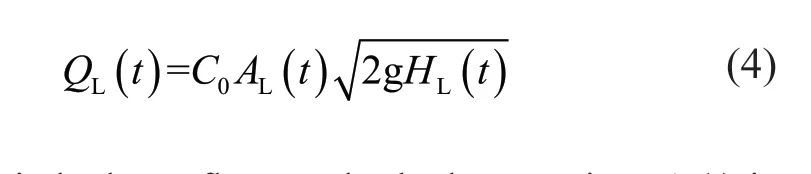
whereQL(t) is leakage flow at the leakage point;AL(t) is the leakage area;HL(t) is water pressure at the leakage point; g is gravitational acceleration;tis time; andC0is a model parameter, which can take a value of 0.06-0.12 for a rigid joint and 0.03-0.06 for a flexible joint (Liuet al., 2014).

For any joint in a pipe network, the leakage area of this joint can be estimated as follows (Liuet al., 2014):

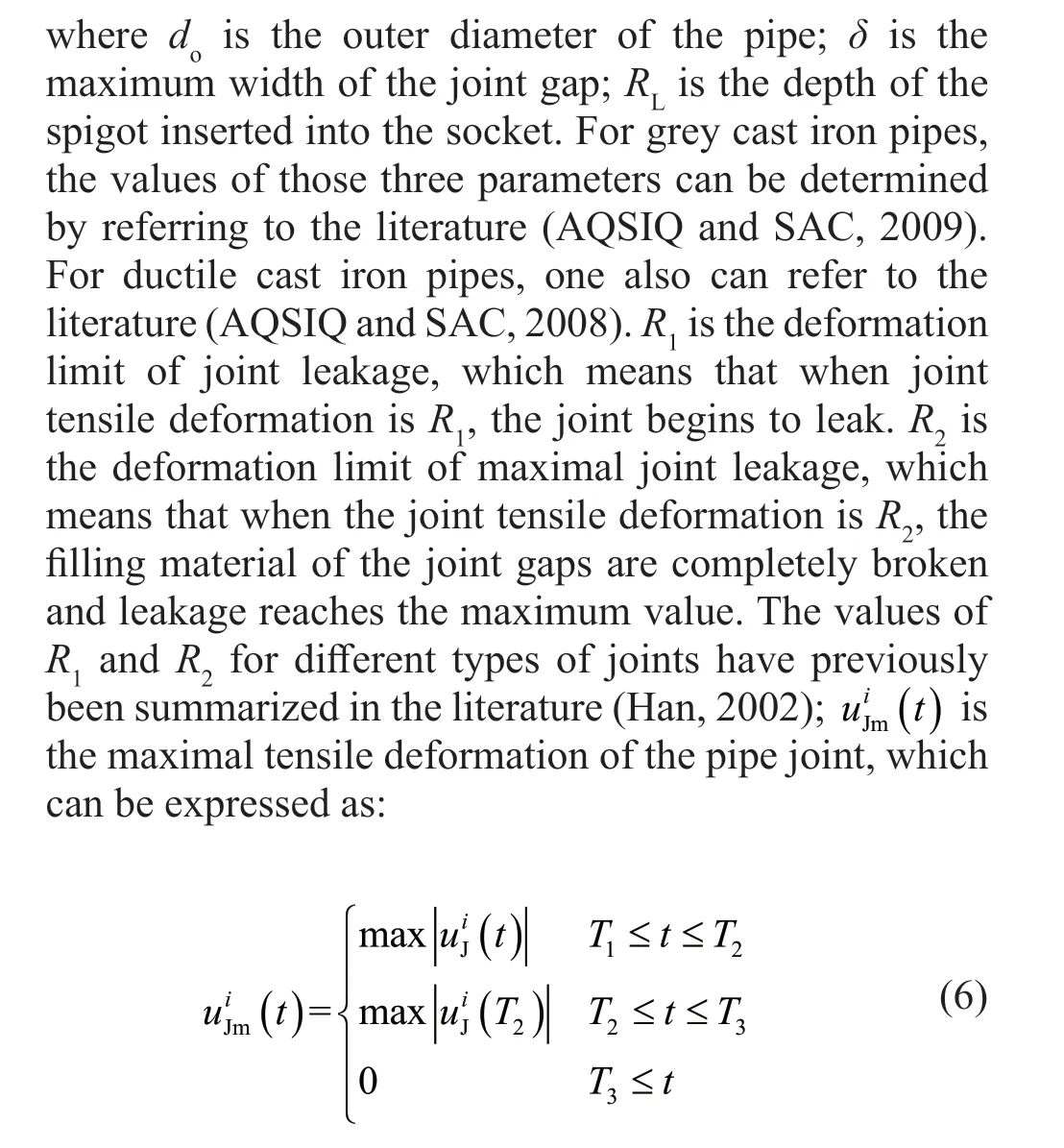
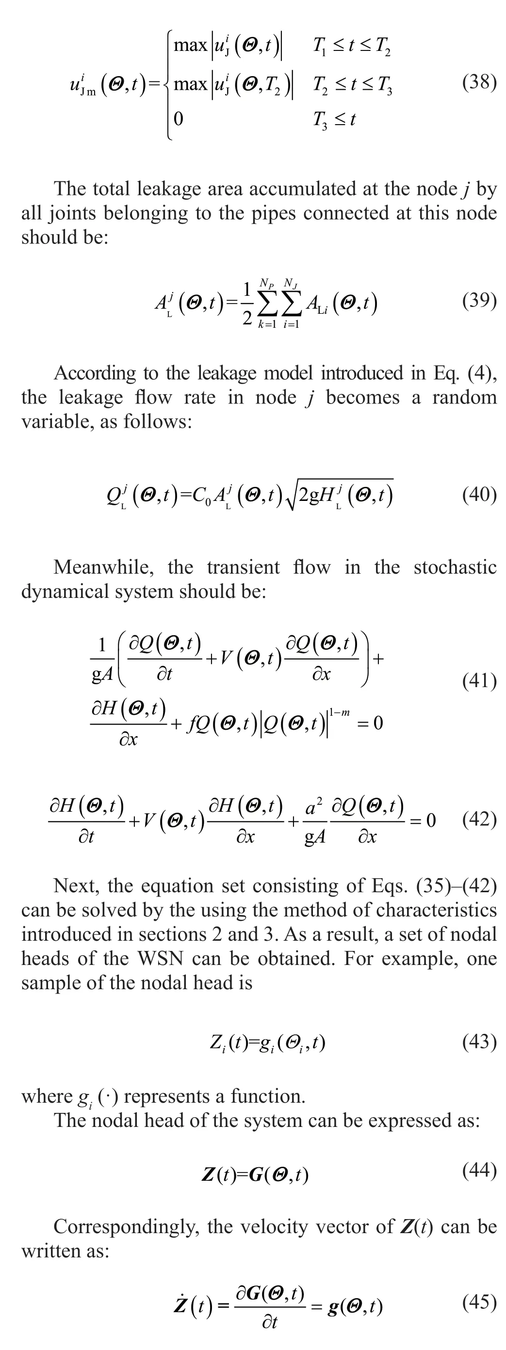
whereT1andT2are the beginning and ending time of the earthquake; andT3is the time at which the broken joint has been repaired.

For simplicity, we assume that the leakage area of all joints in a pipe can be centralized at its ends. This is because there are numerous joints in a WSN. Modeling and analyzing each leakage point are unrealistic.Therefore, for nodejin the pipe network, the total leakage area for this node should be:

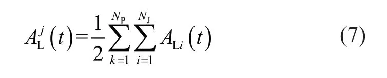
whereNJis the number of the joint of pipek, andNPis the number of pipes at nodejin the pipe network.

4 Transient flow analysis in pipe networks

To measure transient flow in pipe networks, the transient flow analysis method in single pipes and pipe networks with complicated topological structures is introduced in detail as follows.

4.1 Transient flow in a single pipe

For one-dimensional transient flow in a single pipe, as shown in Fig. 3, its momentum equation and continuity equation can be respectively expressed as(Chaudhry, 2014):

where g is the acceleration of gravity;APis the crosssectional area of the pipes;Qis the flow rate in the pipe;Vis the fluid velocity;His the water head; andfandmare two coefficients of friction resistance, which depend on different hydraulic loss models. Generally,ais the propagation velocity of small disturbances, such as sound, which can be expressed as (Chaudhry, 2014):

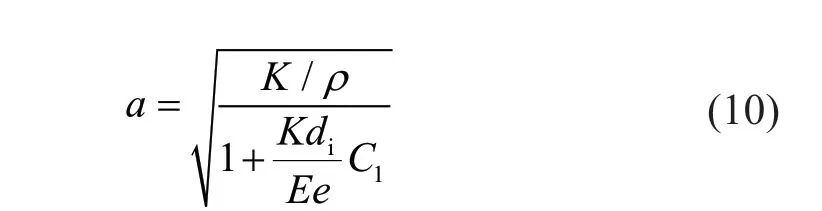
whereKis the bulk modulus of the fluid;ρis fluid density;diis the inner diameter of the pipe;eis the wall thickness of the pipe; andC1is a parameter, which depends on the support conditions of pipe ends. When one end of a pipe is fixed, the other can lengthen and shorten freely, soC1should be 1-μ/2,whereμis the Poisson′s ratio. When both ends of the pipe are fixed,C1is 1-μ2. In addition,when the pipe can lengthen and shorten freely at both ends,C1is equal to 1.

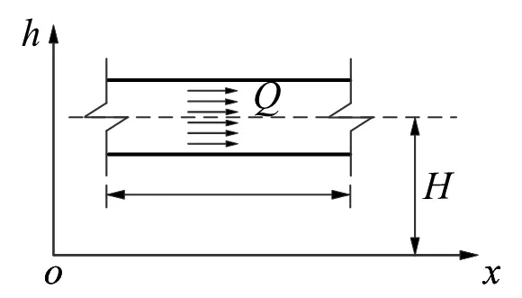
Fig. 3 One-dimensional flow in a pipe

The method of characteristics can be used to solve the above differential equations. In this method, the pipe can be divided intoNparts and the number of the nodes is 1, 2…,N,N+1. At the same time, the computation timeTalso is divided intonparts and we can obtainn+1 moments, namely 0, 1, 2…,T-Δt,T,where Δtis the time interval. Then, in thex-tplane, the finite difference equations will be:

where point P is the point whose information, including pressure and flow rate, needs to be solved at that very moment, as shown in Fig. 4. Points A and B are two points next to point P whose information had already been garnered at the last moment.HPandQPare the pressure and flow rates of point P.RA,RB,SA,SBare four parameters arrived at according to the information pertaining to points A and B, which can be expressed as:

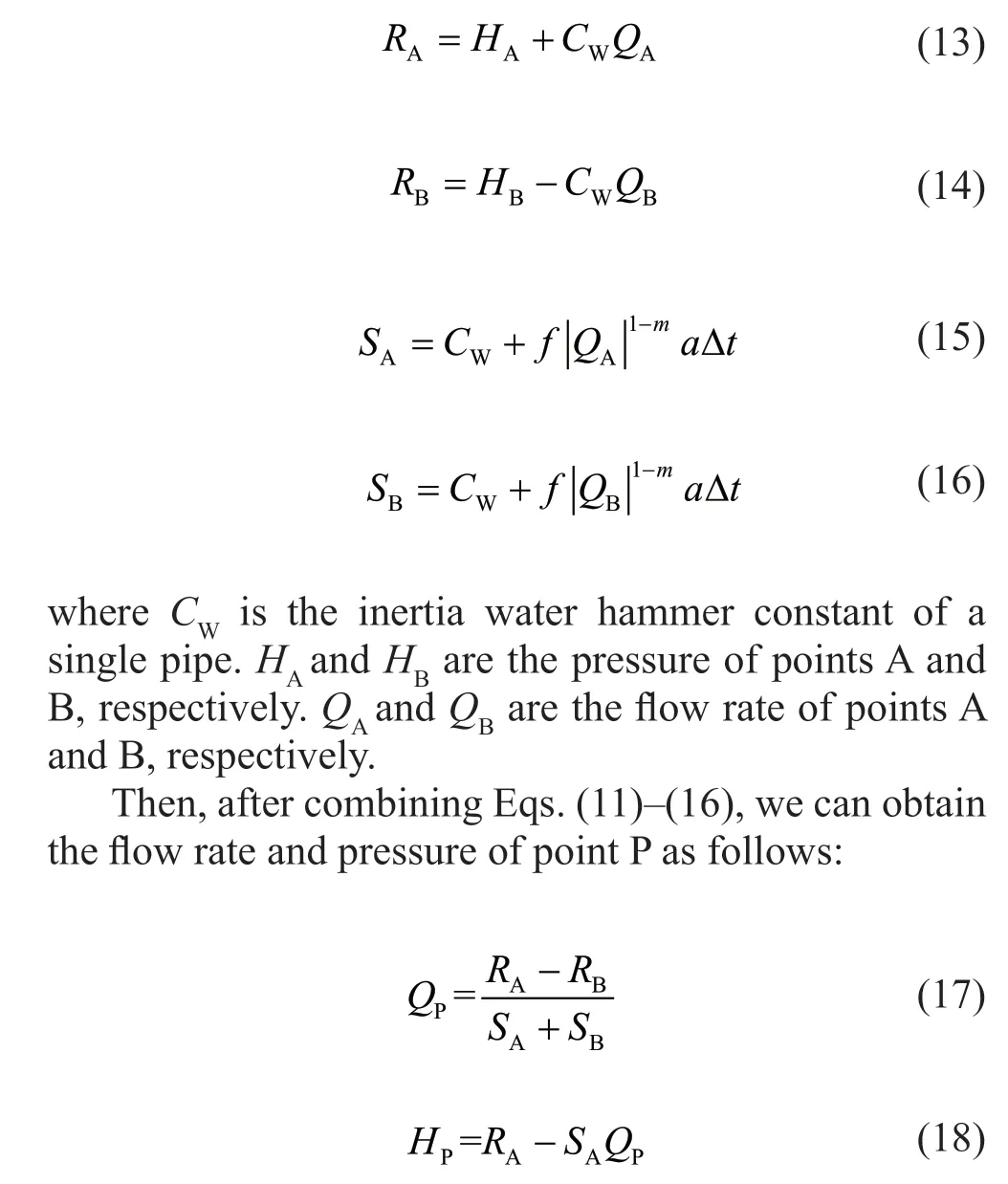
Of course, for transient flow in a single pipe, we still must consider different boundary conditions. The common ones include constant pressure boundary,constant flow rate boundary, downstream valves and so on. More detailed information can be referred to in the literature (Chaudhry, 2014).

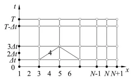
Fig. 4 Method of characteristics

4.2 Transient flow in pipe networks

An actual WSN consists of straight pipes and deformed pipes, such as elbows, tees, crosses and other fittings. When we analyze the transient flow of a pipe network, two problems must be solved. The first is how to divide all pipes in a network into different integer parts. This can be solved by adjusting the wave velocity in different pipes. The second is the relationship between dynamic water pressure and flow rate in different pipes.The following method is utilized for the second problem:

Herein, a node connecting two pipes is analyzed as an example. For other more complicated cases, a similar strategy can be used. It is supposed that pipesiandjconnect with each other, as shown in Fig. 5 and that the water pressure and flow rate at timenΔtare already known. Then based on the method of characteristics, at the junction of two pipes we have:

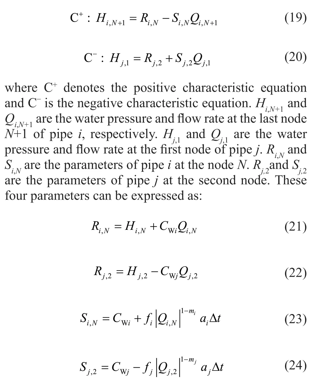
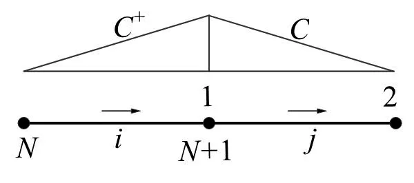
Fig. 5 Connection point between two pipes

whereHi,NandQi,Nare the water pressure and flow rate at nodeNof pipei, respectively.Hj,2andQj,2are the water pressure and flow rate at the second node of pipej, respectively.CWiandCWjare the inertia water hammer constant of pipesiandj, respectively;fiandfjare friction coefficients of pipesiandj, respectively;miandmjare the parameters in the friction loss model of pipesiandj, respectively; andaiandajare the wave velocities of pipesiandj, respectively. At the same time, at the common node the energy equation and the continuity equation should be:

4.3 Transient flow in pipe networks with leakage

Buried pipe networks will be damaged to varying degrees by earthquakes. The leakage area of different nodes can be obtained according to Eq. (7). At the same time, the relationship between the leakage flow rate and the water pressure has already been shown in Eq. (4). herein,the transient flow in two pipes with leakage can be determined according to the following equation, while in other more complicated cases a similar solution can be obtained.

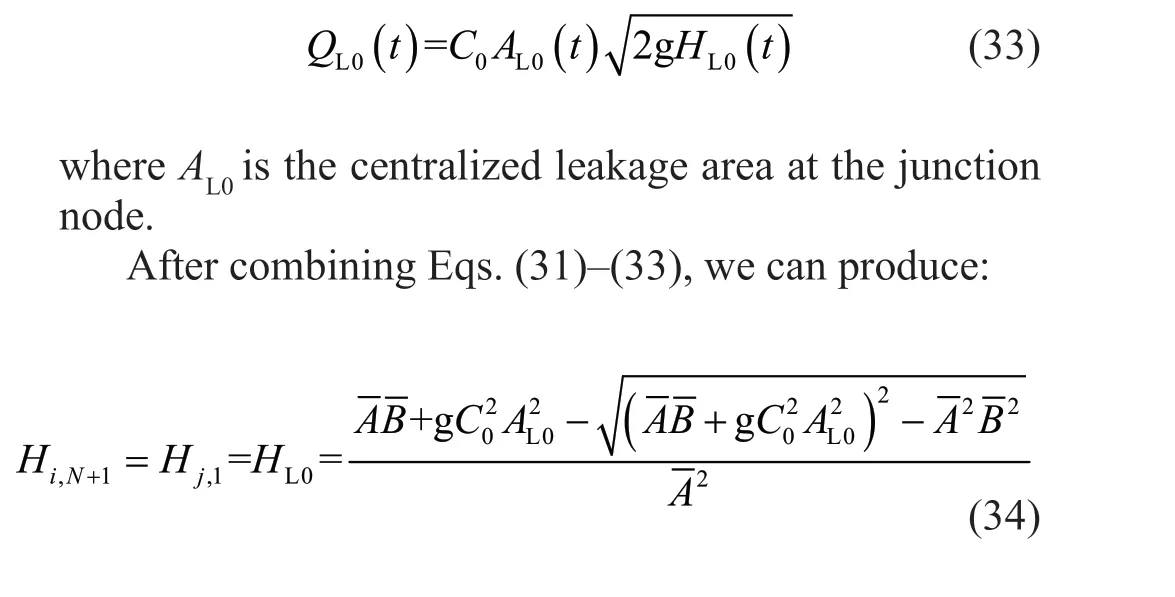
For the two pipesiandj, as shown in Fig. 6, the positive and negative characteristic equations are shown in Eqs. (19) and (20). Then at the junction, based on the equilibrium conditions of water pressure and flow rate,we can stipulate:

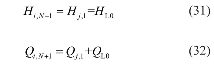
Fig. 6 Hydraulic solution of WSNs with leakage

whereHL0andQL0are the water head and leakage flow at the common node of pipesiandj, respectively.

Meanwhile, the leakage flow at the junction node should be:

5 Seismic serviceability of WSNs via PDEM

5.1 Stochastic nodal head in WSNs

We use the probability density evolution method(PDEM) to analyze the seismic serviceability of a WSN.The stated equation of the pipe-soil-water system must first be established. For the buried pipe network in a random ground motion field, the motion equation of the network is expressed as follows:

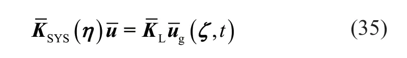
whereη=(η1,η2,...,ηs1) represents the random vectors in the buried pipe network andζ=(ζ1,ζ2,...,ζs2) represents the random vectors in ground motions, in whichs1 ands2 are the number of random variables of the pipe network and ground motions, respectively. The two types of random variables can be integrated into one random vector asΘ=(η,ζ)=(η1,η2,...,ηs1,ζ1,ζ2,...,ζs2)=(Θ1,Θ2, ...,Θs), in whichs=s1+s2 is the number of random variables of the system .

Further, the axial joint deformation of pipes can be written as:

whereG1(Θ,t) are the function of random variablesΘand time.

Then the random leakage area of a joint can be expressed as:

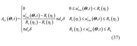
where

For the stochastic dynamic system described by Eqs.(35)-(42), all of its randomness comes from the vectorΘ. Therefore, according to the principle of probability conservation, the augmented system (Z(t),Θ) is also a probability conservation system. Its joint probability density function ispZΘ(z,θ,t). Further, the joint probability function should satisfy the following probability density evolution equation (PDEE) (Li and Chen, 2009):

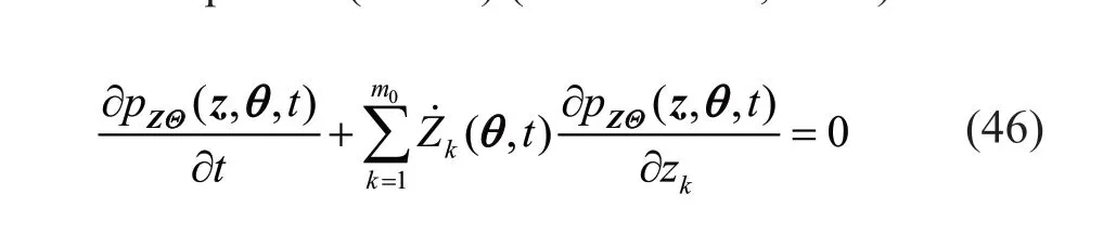
wherem0is the number of the target physical parameters.The initial condition of Eq. (46) can be specified as follows:

whereδis the Dirac function,z0is a deterministic initial vector, andPΘ(θ) is the joint PDF ofΘ.

The solution for PDEM is a process of combing the physical function with the PDEE. Numerical solution methods are necessary for most engineering problems.After solving for the PDEE, the PDF ofZ(t) is derived from:

5.2 Dynamic reliability of nodes

Generally, the performance function of different nodes can be defined as:

whereZi(t) is the dynamic water head of nodei; Zlim,i(t)is the demand water head of the nodei,which usually can be seen as a constant; andiis the number of different nodes and takes a value of 1, 2, 3,…,N0(N0is total number of customer nodes in the WSN).

When the stochastic seismic response of the nodal head has been obtained according to Eqs. (41) and (42),nodal dynamic reliability can be further expressed as:

5.3 Global dynamic reliability of WSNs

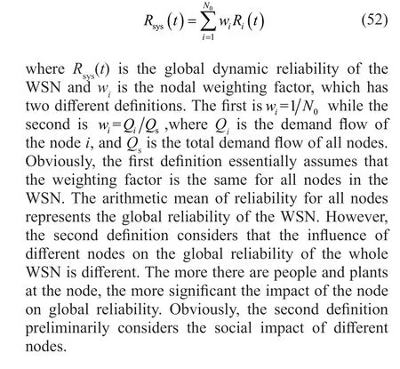
For consumers, perhaps they are most concerned about the functions of the nodes related to themselves.However, for the managers of the entire WSN, or government officers, or other decision-makers, they are more concerned about the seismic performance of the entire system. Therefore, an index referred to as the global dynamic reliability of the WSN can be defined as:

5.4 Basic steps of the suggested method

To evaluate the dynamic seismic serviceability of WSNs based on the method suggested above, the basic steps can be summarized as follows:

(i) Select representative pointsθqin the random parameter spaceΩΘand then assign the corresponding probabilityPqto the pointθq, whereq=1, 2,...,N.Nis the number of selected points. (ii) For the representative pointθq,Nsamples of ground motion fields can be obtained. Then the WSN should be calculatedNtimes and the leakage area ofNsamples of the WSN can be obtained. Furthermore, Eqs. (40)-(42) are solved to obtain the nodal head. (iii) Then for the selected pointθq, the PDEE can be obtained and solved using the finite difference method. (iv) Synthesizing the results will yield the instantaneous PDF as shown in Eq. (48).(v) Based on the basic demand water head of different nodes, calculate the nodal reliability according to Eq.(51). (vi) According to the weighting factors of different nodes, the global reliability of the WSN can be obtained according to Eq. (52).

6 Case study

To further explain the method suggested in this paper, an actual WSN in Mianzhu is studied. In this paper, the topological distribution of the network, the material and geometric properties of the pipelines, such as their diameter and length, are all known. Limited by the length of the paper, they are not listed in detail. For the pipeline age, we do not yet have valid data.

The layout of the WSN, including the number of nodes, pipes, and water sources, is shown in Fig.7. Herein, there are 118 nodes and 139 pipes. Nodes 115-118 are for four water plants, and the water head is set as 41 m. Nodes 1-114 are actually 114 sink nodes.The total pipe length is about 47 km, including 7 km of grey cast iron pipes, 26 km of prestressed concrete pipes and reinforced concrete pipes, 10 km of ductile cast iron pipes and polyethylene pipes. Additionally, there are about 0.38 km of steel pipes. During the Wenchuan earthquake, 70% of the main pipes were damaged. The leakage rate increased from 17% before the earthquake to 85% after the earthquake. Much nodal head decreased heavily, even to zero (Liuet al., 2015b).

The geotechnical investigation showed that the mean shear wave velocity was about 300 m/s.Therefore, according to the Chinese seismic design code(GB 50032-2003, 2003), the WSN was located in the type II site. In addition, the seismic investigation showed that in Mianzhu the damage intensity was about VIII(Caoet al., 2011). Therefore, the peak value of seismic accelerations was set to 0.20 g (GB 50011-2010, 2010).

6.1 Modeling and stochastic seismic response of WSNs

To ascertain the response of buried pipe networks under the influence of earthquakes, the first step is to build a finite element model of the WSN via the method described in section 3. After discretization, there are 15,479 elements containing 4,577 joint elements and 15,458 nodes.

Fig. 7 Layout of the WSN in Mianzhu

Different from general building structures, lifeline engineering systems are often distributed in space.Therefore, the ground motions imposed on those structures always change spatially. In order to investigate the spatial variant ground motions, researchers have established many different permanent or temporary acceleration arrays, including the SMART-1 array(Abrahamsonet al., 1987), the SMART-2 array (Chiuet al., 1994), and the Chiba Experiment Station in Tokyo (Katayama, 1991). However, there are often two problems when we conduct a random dynamic analysis of lifeline engineering. One is that the shape of the ground motion array is not consistent with the distribution of the studied structure, and the other is that the number of ground motion samples is insufficient.For example, in this study, it is far from enough to conduct a random analysis of the water supply network in Mianzhu based on the acceleration record taken from the Wenchuan earthquake. To this end, we adopted the spatial variant ground motion model proposed by Wang and Li to generate a large amount of time history data of acceleration samples (Wang and Li, 2012). The model can be expressed as:

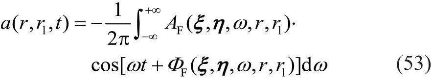
wherea(r,rl,t) is the time history of the ground motion in the engineering site;ris the distance from the hypocenter to the geometric center of the local site;rlis the location of the ground motion in the local site;AF(ξ,η,ω,r,rl)is the amplitude spectrum of the ground motion;ΦF(ξ,η,ω,r,rl) is the phase spectrum of the ground motion;ξ=[A0,T,ωg,ζg,α0,cg]Tis a stochastic vector that represents the factors that affect the ground motion;andη=[K,a′,b′,c′,d′]Tis a deterministic vector, which reflects the effect of transmission paths when the seismic waves propagate from the source to the engineering site. The seismic waves propagate at an angle of 22.7°with respect to the east orientation, from southwest to northeast, considering the location relationship between Mianzhu and the seismic source as shown in Fig. 7.

In this paper, we only consider the randomness of ground motions while the randomness of the water supply network is neglected. The layout of the network is treated in a deterministic manner. However, it should be noted that the ground motions must be variable within the spatial range of the pipe network distribution.

One hundred and fifty sample points are selected according to the GF-discrepancy method (Chenet al.,2016). Then 150 ground motion fields are generated.The duration of ground motions is 10 s. As a result, we can obtain 150 damaged samples for the same WSN.To investigate the damage severity of different samples,the maximal nodal leakage area in different samples is shown in Fig. 8. Accordingly, it is not difficult to find that the damage severity of different samples varies. For example, the maximal nodal leakage area in sample 115 is only 9.8420×10-4m2. The WSN in this sample should be in a slight state of leakage. However, in sample 14, the maximal leakage area of all nodes is as much as 0.1494 m2. The WSN should be in a severe leakage state. Obviously, the randomness of ground motions has an important influence on the damage state of the pipe network.

6.2 Seismic function of WSNs

When the damage state of the pipe network is different, the function of the pipe network is also different. Herein, for the slight leakage state, sample 115 is selected as an example to show the dynamic water head. The water head of nodes 74, 99, and 100 is shown in Fig. 9(a) as an example. Accordingly, the water head will fluctuate slightly under a small leakage state and tends to balance at a small value after a while.For a severe leakage state, for instance, the water head of nodes 74, 99, and 100 in sample 14 is selected, as shown in Fig. 9(b). From Fig. 9(b), it can be found that other than small leakage, the severe leakage evidently affects the nodal head. In sample 14, when leakage occurs, the nodal head of node 100 sharply decreases to zero, while that of nodes 74 and 99 decreases evidently but slowly.Their nodal head changes from 39.35 m and 40.57 m to 23.97 m and 23.88 m, respectively.

Fig. 8 Maximal leakage area of all nodes in different samples

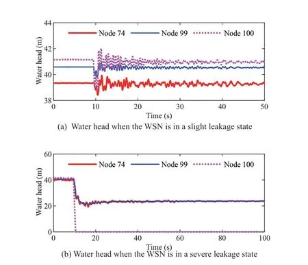
Fig. 9 Dynamic nodal head in the WSN

Then, based on the dynamic water head of different nodes, the PDEE of the water head for different nodes can be solved. Next, the probabilistic information for different nodes can be obtained. The water pressure at node 99 is chosen as an example to demonstrate the results that are shown in Fig. 10.

6.3 Dynamic reliability of nodes

According to the random nodal head and the demand water head, we can reach dynamic nodal reliability based on Eq. (51). When the demand water head is 16 m, the reliability of nodes 74, 99 and 114 is highlighted as an example, as shown in Fig. 11(a).

Fig. 10 Stochastic nodal head at node 99

According to Fig. 11(a), in general all nodal reliability decreases at the beginning of an earthquake,but the changing process of the reliability of different nodes varies. After the beginning of an earthquake, the reliability of node 74 quickly decreases from 1, and when the time is 3.18 s, it decreases to 0.5085. When an earthquake ends at 10 s, its reliability is only 0.1821,which is basically unchanged over time. A similar variation trend for node 99 can be observed; the only difference is the difference in quantity. However, for node 114, reliability fluctuates wildly. Reliability is still 1 at 3.18 s. It begins to decrease at 5.5 s and drops to 0.1821 when the earthquake ends. Obviously, reliability fluctuates. The curve of the reliability is like a sinusoid,with a decreasing amplitude. For example, when the time is 19.66 s and 30.06 s, the reliability of node 114 can increase to 0.9360 and 0.9348, respectively. But reliability decreases slowly and needs more time than that for nodes 73 and 99 to reach a steady state.

Similarly, we can also obtain the dynamic reliability of nodes under a different demand water head. The reliability of node 114 under a demand water head of 10,16, and 22 m is taken as an example and shown in Fig.11(b). Accordingly, it can be found that when the demand water head is 10 m and 16 m, the reliability of node 114 shows significant fluctuation after the beginning of an earthquake. However, when the demand water head is 22 m, the reliability decreases at about 5.5 s and drops to 0.1725 when the earthquake ends (10 s), which is much closer to the value of 0.1658 when the time is 50 s.

6.4 Global reliability of WSNs

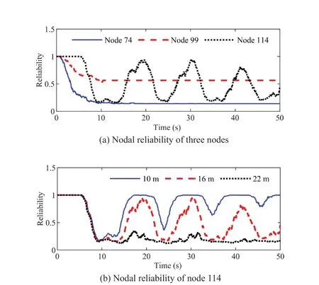
Fig. 11 Dynamic reliability of different nodes

Fig. 12 Global reliability of the whole WSN

Based on the two definitions of nodal weighting factors, we can arrive at two typess of global reliability for the whole WSN. When the demand water head of all nodes is 10 m, there are two types of global reliability,as shown in Fig. 12(a). Accordingly, at the same demand water head, the difference between the two kinds of global dynamic reliability is not so significant. However,with a change of time, the difference between the two kinds of results will fluctuate. For example, when the demand water head is 10 m, bothRsys1(global reliability according to the first nodal weighting factor definition)andRsys2(global reliability according to the second nodal weighting factor definition) are 1 before 0.6 s. Then the difference betweenRsys1andRsys2begins to be prominent.For example, when the time is 10 s,Rsys1is 0.3410 whileRsys2is 0.3975. The latter is 0.0565 larger than the former. The ratio ofRsys1andRsys2is shown in Fig.12(b). Accordingly, it can be found that the ratio is very close to 1. But for most of this period, the ratio is slightly less than 1. This shows that in generalRsys1is less thanRsys2. In other words, when we consider the influence of the reliability of each point on system reliability with equal weight, the calculation result of system reliability is somewhat small, and the analysis result is slightly conservative.

7 Conclusions

This paper suggests a new method for evaluating the seismic serviceability of water supply networks(WSNs). The physical mechanisms of WSNs subjected to earthquakes are introduced in detail to build the analysis framework. Three different physical models are introduced, including a finite element model to capture the seismic responses of WSNs, a leakage model to determine leakage flow, and the transient flow model solved by the method of characteristics to obtain the dynamic water head of different nodes. Then, the stochastic seismic responses of buried pipe networks and the seismic serviceability of WSNs can be obtained via use of the Probability Density Evolution Method.Further, the global reliability of WSNs is suggested by two different definitions of nodal weighting factors.Lastly, an actual WSN in Mianzhu is investigated to show the practicability of the suggested method. The following conclusions can be drawn:

(1) Water flow has a dynamic response during an earthquake. The leakage of joints will affect the nodal water head. The nodal head will decrease sharply at some nodes while it also probably demonstrates drastic fluctuation. When the leakage area of the network is constant, the water pressure and leakage flow rate will gradually stabilize.

(2) The instantaneous probability density function of the dynamic nodal head can be calculated. Therefore,once the demand head of different nodes is determined,the seismic serviceability of those nodes can be obtained.In addition, when the nodal demand head is different, the framework is convenient for evaluating the serviceability of WSNs for people living on different floors.

(3) The randomness from the ground motion field can affect the seismic responses of buried pipes and the leakage state of WSNs. As a result, the dynamic nodal head also displays significant randomness. The framework also provides a dynamic perspective for understanding the spread of randomness from the earthquake field to the water flow in WSNs.

(4) Nodal reliability is a dynamic process directly related to its demand head. Generally, the higher the demand head, the smaller the degree of nodal reliability.

(5) Global reliability supplies a new perspective for estimating the performance of WSNs. Two definitions of nodal weighting factors are suggested to preliminarily consider the social influence of different nodes. The case shows that the difference between two kinds of global reliability is changing over time. Although the difference may be small, its economic influence can be significant.This implies we should establish an appropriate method for estimating the influence of different nodes for the entire network.

In conclusion, the framework provides a new perspective for assessing the dynamic seismic serviceability of WSNs. It not only can evaluate the seismic reliability of different nodes, but can also determine the anti-seismic property of whole WSNs.This would contribute to improving the future design of WSNs for engineers and decision-makers.

Acknowledgement

The support of the National Natural Science Foundation of China (Grant No. 5210082055) and the China Postdoctoral Science Foundation (Grant No.2021M690278) is highly appreciated.