Development of a double-layer shaking table for large-displacement high-frequency excitation

Pan Peng, Guo Youming, Kang Yingjie, Wang Tao and Han Qinghua

1. Key Laboratory of Earthquake Engineering and Engineering Vibration, Institute of Engineering Mechanics,China Earthquake Administration, Sanhe 065201, China

2. Department of Civil Engineering, Tsinghua University, Beijing 100084, China

3. School of Civil Engineering, Tianjin University, Tianjin 300350, China

Abstract: It is difficult to conduct shaking table tests that require large-displacement high-frequency seismic excitation due to the limited capacity of existing electrohydraulic servo systems. To address this problem, a double-layer shaking table(DLST) is proposed. The DLST has two layers of one table each (i.e., an upper table and lower table) and aims at reproducing target seismic excitation on the upper table. The original signal is separated into two signals (i.e., a high-frequency signal and low-frequency signal) through a fast Fourier transform/inverse fast Fourier transform process, and these signals are applied to the two tables separately. The actuators connected to different tables only need to generate large-displacement low-frequency or small-displacement high-frequency movements. The three-variable control method is used to generate large-displacement but low-frequency motion of the lower table and high-frequency but small-displacement motion of the upper table relative to the table beneath. A series of simulations are carried out using MATLAB/Simulink. The simulation results suggest that the DLST can successfully generate large-displacement high-frequency excitation. The control strategy in which the lower table tracks the low-frequency signal and the upper table tracks the original signal is recommended.

Keywords: double-layer shaking table; large-displacement high-frequency excitation; electrohydraulic servo system;three-variable control; MATLAB/Simulink

1 Introduction

The shaking-table test is one of the most important methods in earthquake engineering research (Williams and Blakeborough, 2001). By reproducing earthquake ground motion, the shaking-table test is widely used in the investigation of structural dynamic properties, structural seismic behaviors, and structural failure mechanisms(Xueet al., 2019; Yuet al., 2010; Louet al., 2004).Shaking tables have a long history of development. The earliest known shaking table was constructed in Japan at the end of the 19th century (Severn, 2011). The first usable record from a real earthquake became available in 1936 (Ruge, 1936). Servo-valve control was applied to shaking tables in the mid-1960s. Since then, shakingtable tests have been widely used and more shaking tables were built (Blostotskyet al., 2010; Tsaiet al., 2010).In the mid-1970s, a 5 m × 5 m six DOF shaking table was built in the Federal Republic of Germany (Severn,2011). The world largest shaking table, which has a size of 20 m × 15 m, was completed at E-Defense in 2005(Ohtaniet al., 2003). Currently, the further development of shaking tables is focused on two issues: large scale and table array (Wanget al., 2005).

Among the different types of currently existing shaking tables, the electrohydraulic shaking table(EHST) with hydraulic actuators is most actively used in situations that require strong actuating forces (Tanget al., 2016). However, one of the major drawbacks of the EHST system is the strongly nonlinear behaviors of the system (Basileet al., 2009); for example, dead zone,backlash and friction (Yaoet al., 2008). Hence, highly accurate control of an EHST system remains challenging and various control methods have been proposed to improve tracking performance.

EHST systems have traditionally been displacement controlled by classical proportional-integral-differential control algorithms. The proportional-integral-differential controller performs well in the low-frequency range but its tracking accuracy decreases over a certain frequency. To extend the bandwidth of the system and improve tracking accuracy, Tagawa and Kajiwara (2007) developed a three-variable control (TVC) method and applied it to EHST control. A TVC controller simultaneously uses displacement, velocity, and acceleration for control and thus realizes sufficient accuracy at all frequencies. TVC controllers are therefore widely used in EHST systems and have been well verified in practice.

Researchers have proposed other control methods.Spencer and Yang (1998) proposed the transfer-function iteration method and verified it by a linearized model.This method can improve tracking performance by adjusting the command signal. The command signal can be obtained using an inverse transfer function and is iteratively modified offline until the desired tracking accuracy is obtained. Shenet al. (2011) combined adaptive inverse control and a technique of equalizing inverse frequency response functions, achieving better accuracy of time waveform replication. Enokidaet al.(2014) proposed nonlinear signal-based control that comprises online feedforward compensation and offline feedback compensation. This method was examined using numerical examples in MATLAB/Simulink and has the most accurate input identification in all linear and nonlinear cases. Nakata (2010) proposed a method of acceleration trajectory tracking control that involves an acceleration feed-forward controller, a system dynamics command compensator, and an actuator displacement feedback controller. Phillipset al. (2014) proposed a model-based multi-metric shaking-table control strategy that is robust against nonlinearities, including changes in specimen conditions. Chenet al. (2017) incorporated a feedback controller into a weighted commandshaping controller. The control command issued to the shaking table is the weighted summation of the shaped displacement and acceleration. The mentioned methods have been shown to have better control accuracy and/or robustness for conventional EHSTs; however, there has been little development of new types of shaking tables.

In 2010, the Kajima Corporation built a double layer shaking table called the W-DECKER to test the substructures of skyscrapers (MTS Systems Corporation, 2010). The W-DECKER has an extremely long stroke shaking table above a normal main shaking table. Therefore, it can reproduce the long-period seismic responses of the skyscrapers. The idea of the W-DECKER is innovative, and its application to skyscrapers was successful. However, the applicability of W-DECKER to large scale structures, which are sensitive to excitations with a large displacement and a wide frequency band, has not been investigated.

In recent years, many more large-scale structures have been built or are about to be built; e.g., large-span domes and water hydraulic dams. Shaking-table tests for these important and complex structures are necessary. In these cases, the shaking tables need to be large enough to reduce scale effects. Due to the complexity of such structures, high-frequency excitation is needed to consider higher modes of the specimens. Large-displacement excitation is also needed to obtain the dynamic response of structures subjected to near-fault ground motion.However, the actuator can generate large-displacement movements but will struggle to generate high-frequency movements if it has a long stroke, while it can generate high-frequency movements but will struggle to generate large-displacement movements if it has a short stroke.Conventional EHSTs use one or multiple actuators acting in a certain direction, and it is thus difficult for them to generate excitation that is simultaneously of large displacement and high frequency.

The present study proposes a double-layer shaking table (DLST) that has two layers of one table each.The excitations are separated into two parts in the frequency domain, which are separately applied to the two tables. The actuators connected to the lower table only need to generate large-displacement lowfrequency movements whereas those connected to the upper table only need to generate small-displacement high-frequency movements. In this study, the concept and dynamic model of the DLST is presented first.Models of the conventional EHST and proposed DLST equipped with electrohydraulic servo systems and TVC controllers are then built using MATLAB/Simulink. A series of simulations are then carried out to verify the effectiveness of the DLST in terms of generating largedisplacement and high-frequency excitation.

2 Development of the DLST

2.1 Concept of the DLST

The excitation model of a conventional shaking table is shown in Fig. 1 (Phillipset al.,2014). The complete and full-frequency excitations are applied by one or multiple actuators. Figure 2 shows the excitation mode of a DLST with two tables and two actuators. The two tables are connected by an isolation layer and are actuated by the respective actuators independently. The lower actuator, which is designed for low-frequency large-displacement seismic excitation, is set between the lower table and the reaction wall. The upper actuator for high-frequency small-displacement seismic excitation is set between the two tables. If the lower table provides low-frequency motion and the upper table provides highfrequency motion relative to the table beneath, the upper table is expected to generate complete seismic excitation with full-frequency components. In addition, the upper table can sometimes be removed to let lower table work as a normal large-scale shaking table.

The original input signal of seismic excitation is separated in the frequency domain to obtain a highfrequency signal and a low-frequency signal. The two tables are controlled by two TVC controllers. There are two control strategies that can be selected. (1) The lower TVC controller instructs the lower table to track the low-frequency signal while the upper TVC controller instructs the upper table to track the original signal with all frequency components. (2) The lower TVC controller instructs the lower table to track the low-frequency signal while the upper TVC controller instructs the relative displacement between the upper table and lower table to track the high-frequency signal. The performance of the two control strategies are compared in Section 4.

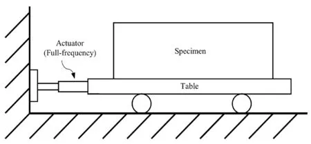
Fig. 1 Excitation model of the conventional shaking table

Fig. 2 Excitation model of the DLST

Figure 3 is a block diagram of the DLST. The input signalais separated though a fast Fourier transform(FFT) and inverse fast Fourier transform (IFFT) process.Two signals1aanda2are then input to corresponding TVC controllers. The two controllers provide drive currentsI1andI2to the two electrohydraulic servo systems. The electrohydraulic servo systems then generate forces1Fand2Fto actuate the two tables. The displacements, velocities, and accelerations of the two tables can be measured in real time and are transmitted back to the corresponding TVC controllers, which realizes close-loop control.

Compared with the existing double table system W-DECKER (MTS Systems Corporation, 2013), the proposed DLST has a major difference. The W-DECKER is designed for testing substructures of skyscrapers and the major contribution of the system is on how to achieve an extremely long stroke. The W-DECKER consists of a long stroke table placed above a short stroke table.The shaking table proposed herein, i.e., the DLST, is designed for testing large-scale structure models with different scale ratios, such as water hydraulic dams and long-span domes, and the major contribution is on how to realize the excitation with a large displacement and a wide frequency band. The DLST consists of a short stroke table placed on a long stroke table. The control of the proposed shaking table is much more difficult than that of the W-DECKER. This is because in the W-DECKER, the short stroke actuator is used to control the lower table, and it can generate both low-frequency and high-frequency excitations. The short stroke actuator can easily provide reaction forces for the upper table′s movement, which only has low frequency components,thus the conventional control strategies can be used for the control. Whereas in the proposed shaking table, the long stroke actuator is used to control the lower table,and it can only generate low-frequency excitation. It is difficult for the long stroke actuator to provide highfrequency reaction force for the upper table′s movement,thus much more advanced control strategies are needed to achieve accurate control. In summary, the two table systems are developed for different application scenarios,and aim at resolving different challenges.

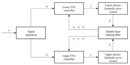
Fig. 3 Block diagram of the DLST

2.2 Dynamic model of the DLST

The dynamic model of the DLST is built in MATLAB/Simulink using Eqs. (3) and (4) as shown in Fig. 5. In the figure, two modules (i.e., Mux and Demux provided by MATLAB/Simulink) are used to combine and decompose signals.

3 Control of the DLST

3.1 Modeling of an electrohydraulic servo system

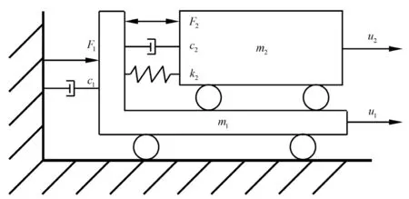
Fig. 4 Simplified dynamic model of the DLST

Figure 6 shows the structure of an electrohydraulic servo system that includes a servo valve and actuator.As shown in the figure,1Pand2Pare pressures in the two chambers,1Vand2Vare the volumes of the two chambers,1Qis flow into chamber 1, and2Qis flow out of chamber 2. The servo valve can be described as a second-order system between the drive currentIand the spool displacement of the servo valvexv. The transfer function can be expressed as

Fig. 5 Simulink model of the DLST

whereKv,vω, andvξare, respectively, the gain coefficient, natural angular frequency, and damping ratio of the servo valve.

The relationship between the flowQand the servo valve spool positionxvcan be linearized as

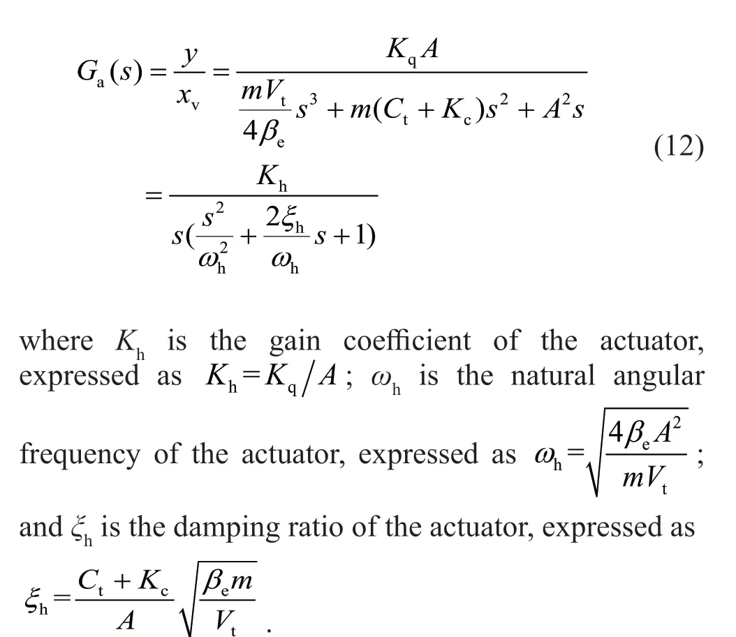
The transfer function from the servo valve spool positionvxto the piston positionycan be obtained using Eqs. (9), (10), and (11):

The model of the electrohydraulic servo system is built using Eqs. (5), (9), (10), and (11) in MATLAB/Simulink, as shown in Fig. 7. The model needs a drive current as an input signal and outputs a force to actuate the table. The measured velocity of the table is sent back to the electrohydraulic servo system to form a small loop. The model introduced in this section is for a single electrohydraulic servo system, which is commonly used in conventional shaking tables. The DLST model combines several parts and is introduced in Section 3.3.

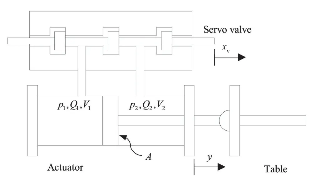
Fig. 6 Structure of electrohydraulic servo system

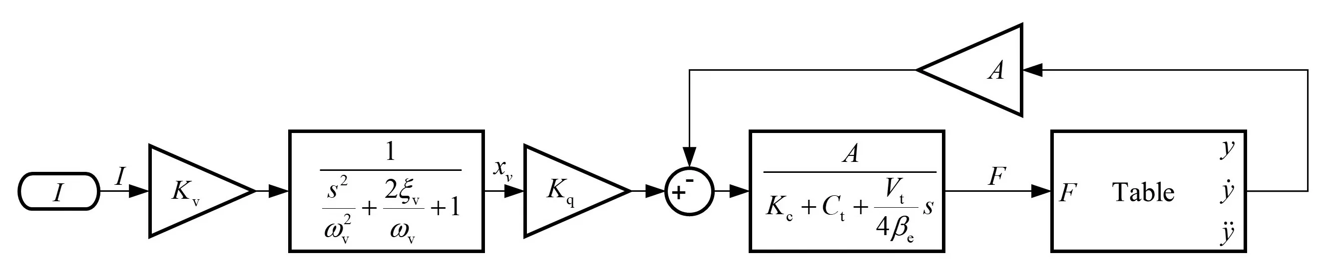
Fig. 7 Simulink model of the hydraulic servo system

3.2 Design of the TVC controller

Figure 8 shows the structure of a TVC controller for a conventional EHST (Tagawa and Kajiwara, 2007). A TVC controller can be divided into three parts, namely a signal generator, feedforward, and feedback. Eight parameters need to be determined before testing and are kept unchanged during the test; specifically,dsgandvsgare determined for the signal generator,Kaff,KvffandKdffare determined for the feedforward, andKafb,KvfbandKdfbare determined for the feedback. The design of the feedforward is based on the design result of the feedback,and the feedback therefore needs to be designed before the feedforward. The design of the signal generator is independent of the other two parts.

3.2.1 Design of the signal generator

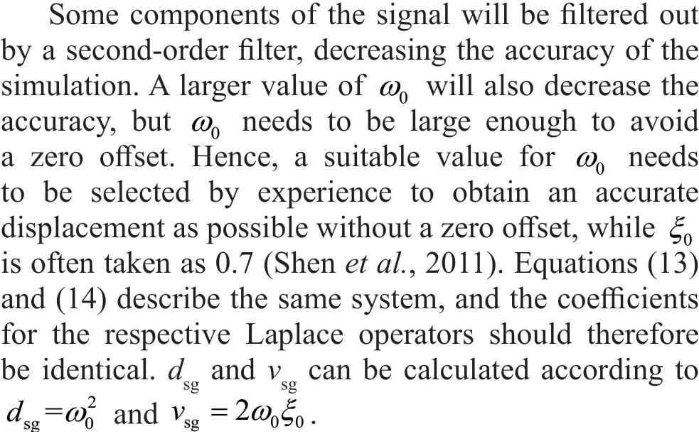
The design of a TVC controller is based on a displacement closed loop, while seismic ground motions are recorded as a time history of acceleration. A signal generator is thus needed to transfer the acceleration signalarefto the displacement signaldrefwithout zero offset. A velocity feedback and an acceleration feedback are used to solve the zero-offset problem and the transfer function for the signal generator can be written as

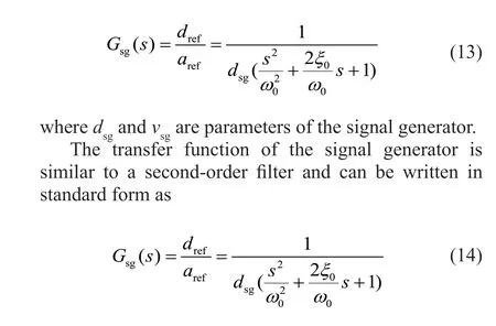
where0ωand0ξare the natural angular frequency and damping ratio of the signal generator.

3.2.2 Design of the TVC feedback

An electrohydraulic servo system can be described by Eqs. (5) and (12) in series. The transfer function can be obtained as

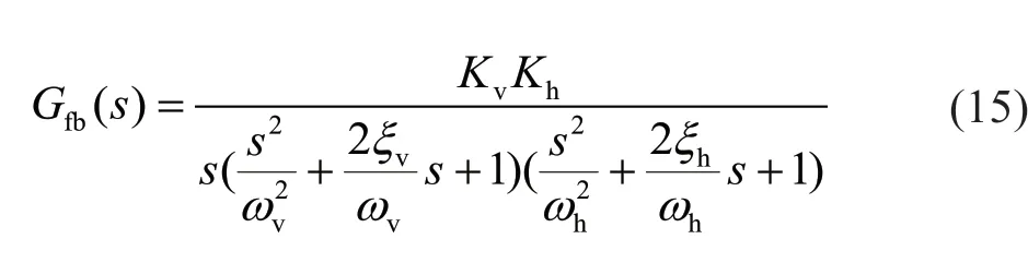
whereωv,ξv, andKvare the parameters of the servo valve whileωh,ξh, andKhare the parameters of the actuator.These parameters represent the inherent properties of the system and can be obtained by system identification or using Eq. (12).

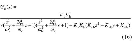
The electrohydraulic system with a feedback part, which is a displacement closed-loop system, can therefore be obtained as

whereKafb,Kvfb, andKdfbare unknown parameters of the TVC feedback to be solved.

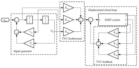
Fig. 8 Simulink model of the TVC controller

The displacement closed-loop system can be transformed to a standard form that comprises three subsystems in series:

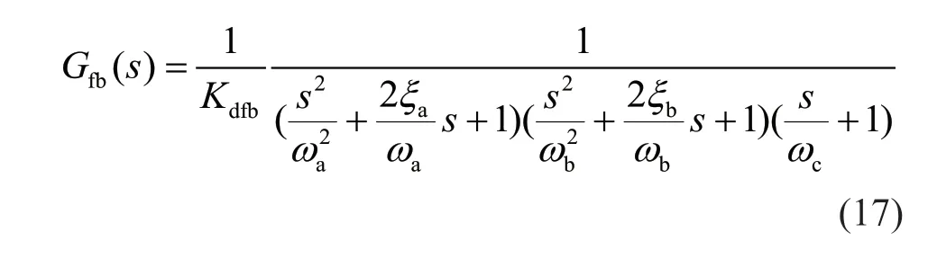
whereωa,ωbandωcare the natural angular frequencies of the subsystems whileξaandξbare damping ratios of the subsystems.

ωais taken as 50rad/s based on experience. The critical damping ratio is 0.7,ξaandξbare commonly taken as 0.5-0.7. In this study,ξaandξbare defined as 0.5 in the simulations. The unknowns in Eq. (17) are thereforeωbandωcwhile the unknowns in Eq. (16)areKafb,KvfbandKdfb. Equations (16) and (17) describe the same system, and the coefficients for the respective Laplace operators should therefore be identical. A set of equations is obtained as

All the control parameters for a single table can be obtained by following the procedure in Section 3.2.The two tables have different parameters, which vary in different cases. Thus, the control parameters need to be calibrated for each table in each case.

3.3 Processing the input signal and modeling the DLST

The present study uses four ground motions recorded for the Taft, Loma Prieta, El Centro, and Kobe earthquakes in the simulations. All the signals are adjusted to have a maximum acceleration of 8 m/s2. The DLST is also expected to test large scale structures, such as water hydraulic dams and long-span domes. Although the table is large, some structures to be tested have to be models with small scale ratios. In a shaking-table test of a scaled model, it is common practice to compress the time axis of the ground motions following the similitude law (Zhang, 1997). For instance, if the time axis is compressed to 1/5 by reducing the sample time,the maximum notable frequency of excitation increases by five times, i.e., from 20 to 100 Hz.

The input signal of a DLST is separated into two signals in the frequency domain; i.e., high-frequency and low-frequency signals. The separation process is shown in Fig. 9 and can be divided into three steps:(1) transferring the acceleration signal to the frequency domain employing the FFT, (2) dividing the frequency spectrum at a certain frequency and obtaining two signals in the frequency domain, and (3) transferring the two signals back to the time domain employing the IFFT. The sum of the high-frequency signal and lowfrequency signal is exactly the same as the original signal. All signals are divided at 15 Hz in the present simulations.

Figure 10 shows the whole model of a DLST, which consists of two shaking tables, two electrohydraulic servo systems, and two TVC controllers. The two shaking tables and electrohydraulic servo systems are encapsulated as sub-models, whose details are shown in Figs. 5 and 7.

4 Simulation

4.1 Parameters and simulation cases

Fig. 9 Process of signal separation

whereTandξare, respectively, the period and damping ratio of the isolation bearing.

The parameters of the electrohydraulic servo systems are defined in accordance with the model in(Huang, 2008), and details are given in Table 1. For the DLST, the upper and the lower systems have the same parameters except for the natural angular frequency of the servo valves, whereωvlrepresents the lower servo valve andωvurepresents the upper servo valve. The servo valve is a second-order system that filters out highfrequency components in signals. The natural frequency thus needs to be high enough to guarantee accuracy. The upper electrohydraulic servo system is used for highfrequency excitation, and its servo valve thus needs a higher natural frequency. For the conventional EHST,the model parameters are the same as for the lower table in DLST.

Fig. 10 Simulink model of the DLST

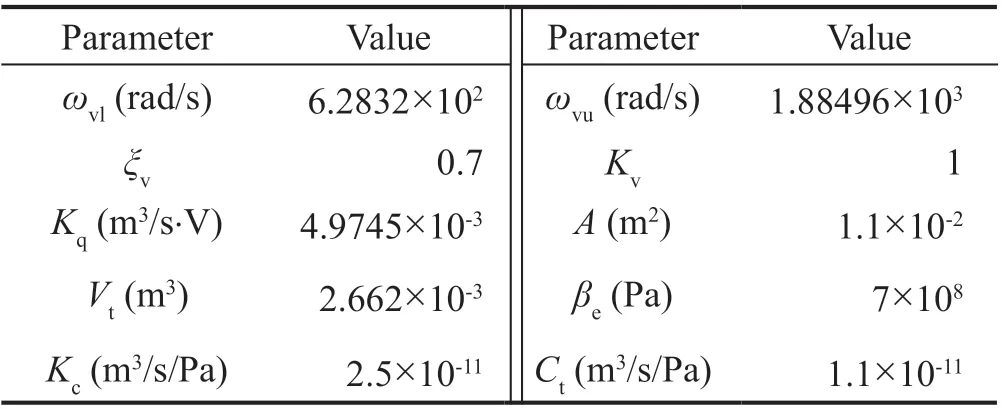
Table 1 Parameters of electrohydraulic servo systems

Table 2 Simulation cases

A series of simulations is carried out using MATLAB/Simulink for the cases listed in Table 2.The valuek0is defined as 1.33 ×107N/m. The mass ratio is changed by changing the combined mass of the upper table and specimen2mand keeping the lower table mass1munchanged. There are three objectives of the simulations: (1) comparing the performance of the conventional EHST and DLST under the same conditions, (2) investigating the effect of the mass ratio of the two parts and the stiffness of the isolation layer,and (3) comparing the performance of the two control strategies mentioned in Section 2.1 and selecting the better strategy.

4.2 Comparison of the conventional EHST and DLST

The EHST is simulated using the model shown in Fig. 8 while the DLST is simulated using the model shown in Fig. 10. Case 3 in Table 2 is used as a simulation example. Control strategy 1 presented in Section 2.1 is adopted and seismic excitation Taft is used in the simulation.

Two demands of the actuators need to be met in the present simulation; i.e., the frequency demand and stroke demand. The frequency demand can be obtained from the output force spectrum of the actuators. The stroke demand is equal to the maximum displacement of the table. Figure 11 shows the spectrum of the actuator′s output force and the displacement of the table for the conventional EHST. As seen in Fig. 11(a), the output force has abundant high-frequency components.Figure 11(b) shows the displacement of the table, which has a maximum value of 60.05 mm. It is difficult for a real electrohydraulic actuator to generate such largedisplacement high-frequency excitation.

Fig. 11 Spectrum of the output force of the actuator and displacement of the table in the case of the conventional EHST

Figure 13 shows the spectrum of the output force of the actuators for the DLST. The lower actuator is designed for low-frequency large-displacement excitation, but its output force has high-frequency components. The upper actuator generates high-frequency movements and exerts a high-frequency reaction force on the lower table, which is finally transmitted to the lower actuator. The lower actuator thus needs to sustain a high-frequency force passively rather than actively exert high-frequency forces. The high-frequency reaction force can be regarded as interference and reduces the tracking accuracy of the lower table, which is discussed in Section 4.3. Figure 13(b) shows the output force spectrum of the upper actuator, which has both highfrequency and low-frequency components. The fullfrequency force acting on the upper table corresponds to full-frequency absolute motion of the upper table.The low-frequency components in the force correspond to low-frequency motion, which is mainly taken care of by the lower table. The high-frequency components in the force corresponds to high-frequency relative motion between the two tables and the upper actuator is set between two tables. Thus, low-frequency components in the output force of the upper actuator have limited effects on the behavior of the upper actuator. The upper actuator focuses on high-frequency excitations and the stroke demand of the upper actuator is small.

For a DLST adopting control strategy 1, the upper table tracks the original signal and the lower table tracks the low-frequency signal. Partial enlarged plots of the output acceleration are shown in Fig. 14, revealing that the acceleration of the upper table has high tracking accuracy while the acceleration of the lower table has visible errors. The root-mean-square (RMS) error of frequency domain acceleration is used to describe the tracking errors:

Fig. 12 Displacement of the tables in the case of the DLST

whereiais the magnitude of the output acceleration at each frequency point,airis the magnitude of the reference acceleration at each frequency point, andarmaxis the maximum value of theari.

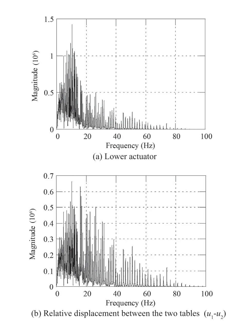
Fig. 13 Spectrum of the output force of the actuator for the DLST

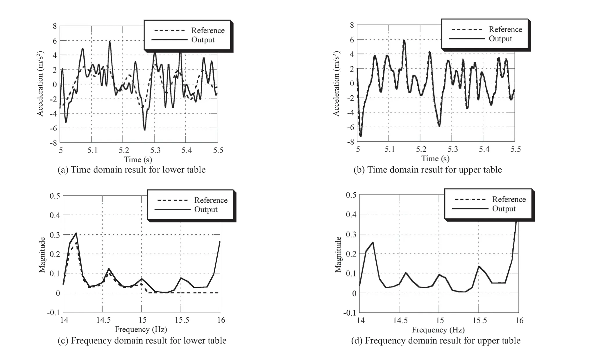
Fig. 14 Partial enlarged plots of the acceleration output of the DLST

The RMS value of the upper table is 0.19% while the RMS value of the lower table is 8.62%. The lower table fails to track accurately while the upper table, which is of most interest, has high tracking accuracy. The reason for the tracking error of the lower table is mainly due to the interaction between the upper and lower tables.

The maximum displacement and frequency band are affected by the time compression ratio of the input signal. Cases 3, 10 and 11 are simulated to further explorer the capacity of DLST when using input signals with different time compression ratios. Note that the original uncompressed signals are used when the time compression ratio is 1. The results are shown in Table 3.When the signals are further compressed, the frequency band becomes wider and the maximum displacement becomes smaller. It can be seen that although the frequency and displacement vary, the upper table always has a small displacement and a high tracking accuracy.

Consequently, for a DLST, the lower actuator only needs to generate low-frequency movements actively and the upper actuator has a small stroke demand, as was expected. The upper table can reproduce the seismic ground motion with high accuracy.

4.3 Effect of parametric variations

Fig. 15 Effect of the mass ratio on the acceleration tracking accuracy

The effect of the mass ratio of the two parts is explored by simulating cases 1 to 5 listed in Table 2.Control strategy 1 mentioned in Section 2.1 is adopted.The acceleration tracking accuracy in these cases is shown in Fig. 15. As the mass ratio increases, the mass of the lower table remains unchanged and the sum mass of the upper table and specimen increases. The upper table thus needs a stronger force for actuation and there is more high-frequency interference of the lower table,which increases the RMS of the lower table. The RMS of the upper table is unaffected by a change in the mass ratio and remains at almost the same small value. The upper table can thus handle the high-frequency tracking error of the lower table by compensating for it in the high-frequency range. Figure 16 presents the output acceleration in the frequency domain when taking seismic excitation Taft as an example. As the mass ratio increases, the acceleration of the lower table has more high-frequency components while the upper table remains unchanged.

Consequently, the motion of the lower table is affected by high-frequency forces transmitted from the upper actuator and the interaction becomes greater when the mass ratio increases. The upper table always has a high tracking accuracy and is not affected by the mass ratio. When the stiffness of the isolation layer is selected within a certain range, it has little effect on the motions of the two tables.

4.4 Selection of a control strategy

All simulations mentioned above used control strategy 1, in which the upper table tracks the original full-frequency signal and the lower table tracks the lowfrequency signal. As previously mentioned, in another control strategy (i.e., control strategy 2), the upper table relative to the lower table tracks the high-frequency signal and the lower table tracks the low-frequency signal. The acceleration tracking accuracy of control strategy 1 is shown in Fig. 15 while that of control strategy 2 is shown in Fig. 18. For control strategy 2,the tracking error of the lower table directly affects the upper table, and Figs. 18(a) and 18(b) thus have the same trend. The RMS acceleration of the upper table is always higher than that when using control strategy 1. When the mass ratio is too large, the RMS acceleration of the upper table increases to an unacceptable value. Figure 19 shows the displacement of the tables for control strategy 2 and seismic excitation Taft. For control strategy 2, the maximum value of1uis 60.19 mm and the maximumvalue of (u1-u2) is 0.55 mm. Compared with the output displacement for control strategy 1 in Fig. 12, the stroke demands of the actuators are slightly smaller but the difference is negligible. Control strategy 1 is a better choice because it has much better tracking accuracy and requires only a negligible increase in the strokes of the actuators.

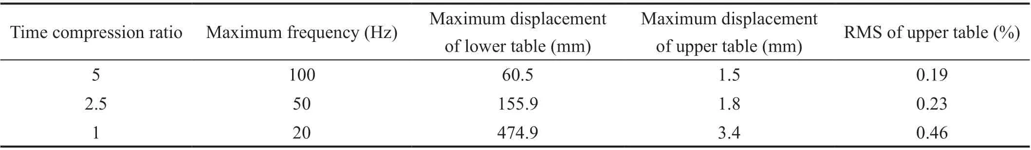
Table 3 Effect of time compression ratio

Fig. 17 Effect of the stiffness of the isolation layer on the acceleration tracking accuracy

Fig. 18 Acceleration tracking accuracy of control strategy 2

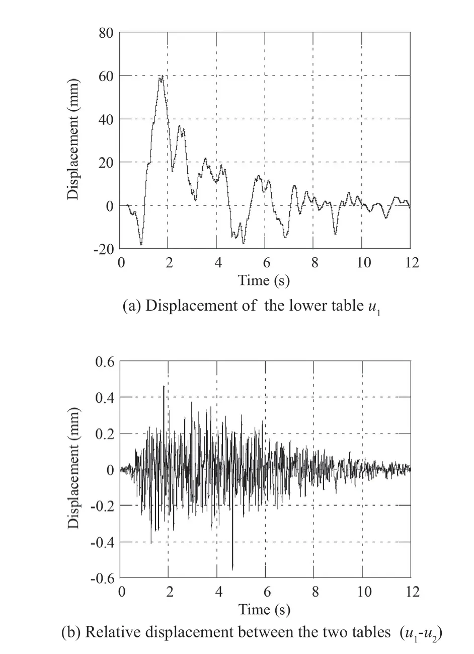
Fig. 19 Displacement of tables for control strategy 2

5 Conclusions

The present study developed a DLST as a new type of shaking table. Simulation models of a conventional EHST and DLST were built using MATLAB/Simulink and a series of simulations were carried out. The major contributions and findings of the study are as follows.

(1) For the proposed DLST, the lower actuator generates large-displacement low-frequency movements while the upper actuator generates small-displacement high-frequency movements. The proposed DLST can reproduce large-displacement high-frequency excitation.

(2) The motion of the lower table is affected by high-frequency forces transmitted from the upper actuator and the interaction becomes greater as the mass ratio increases.

(3) When adopting the right control strategy, the upper table can compensate the tracking error of the lower table and reproduce the target large-displacement high-frequency excitation with high tracking accuracy.

(4) When the stiffness of the isolation layer is selected within a certain range, it has little effect on the motion of the tables. The isolation layer thus does not require special design and can use commonly available isolation bearings.

(5) The control strategy in which the upper table tracks the original full-frequency signal and the lower table tracks the low-frequency signal is a good choice.When using this strategy, the upper table will have high tracking accuracy and a small increase in the required strokes of the actuators is acceptable.

Acknowledgement

The authors are grateful for financial support from the Scientific Research Fund of the Institute of Engineering Mechanics, China Earthquake Administration (Grant No. 2019EEEVL0502), Natural Science Foundation of China (Grant No. 52078275), the Institute for Guo Qiang, Tsinghua University (Grant No. 2019GQC0001),and Beijing Natural Science Foundation (Grant No.JQ18029).