New supervised learning classifiers for structural damage diagnosis using time series features from a new feature extraction technique
2022-01-21MasoudHaghaniChegeniMohammadKazemSharbatdarRezaMahjoubandMahdiRaftari
Masoud Haghani Chegeni, Mohammad Kazem Sharbatdar, Reza Mahjoub and Mahdi Raftari
1. Department of Civil Engineering, Khorramabad Branch, Islamic Azad University, Khorramabad, Iran, 6817816645
2. Faculty of Civil Engineering, Semnan University, Semnan, Iran, 3513119111
Abstract: The motivation for this article is to propose new damage classifiers based on a supervised learning problem for locating and quantifying damage. A new feature extraction approach using time series analysis is introduced to extract damagesensitive features from auto-regressive models. This approach sets out to improve current feature extraction techniques in the context of time series modeling. The coefficients and residuals of the AR model obtained from the proposed approach are selected as the main features and are applied to the proposed supervised learning classifiers that are categorized as coefficient-based and residual-based classifiers. These classifiers compute the relative errors in the extracted features between the undamaged and damaged states. Eventually, the abilities of the proposed methods to localize and quantify single and multiple damage scenarios are verified by applying experimental data for a laboratory frame and a four-story steel structure.Comparative analyses are performed to validate the superiority of the proposed methods over some existing techniques.Results show that the proposed classifiers, with the aid of extracted features from the proposed feature extraction approach,are able to locate and quantify damage; however, the residual-based classifiers yield better results than the coefficient-based classifiers. Moreover, these methods are superior to some classical techniques.
Keywords: structural damage diagnosis; statistical pattern recognition; feature extraction; time series analysis; supervised learning; classification
1 Introduction
There are many civil engineering infrastructures such as skyscrapers, dams, and historical structures that play important roles in the quality of life and social economics. Most of these infrastructures are currently nearing the end of their lives because there are not economic justifications for reconstruction-mentioned systems. Therefore, structural health monitoring (SHM)has recently been paid a great deal of attention by researchers and civil engineers to assess the integrity of structures and detect any potential damage by vibration data (Liet al., 2016; Tanget al., 2019). Damage is deemed to be adverse changes in material and/or geometric characteristics of a structure, which may include changes in boundary conditions and connectivity.These variations seriously affect structural performance and alter the inherent properties of the structure, leading to adverse changes in vibration responses.
The general methodology of SHM is decomposed into four levels, including damage existence detection,damage localization, damage severity, and structural life prediction (Farraret al., 2001). These four levels are normally carried out by model-driven (Entezamiet al.,2017; Hsuet al., 2019; Sarmadiet al., 2020b) or datadriven (Abasiet al., 2021; Avciet al., 2021; Dinget al.,2019; Entezamiet al., 2019; Sarmadi and Yuen, 2021,Zhanget al., 2013) approaches. However, the second category of SHM presents practical approaches to damage detection. This is because of the direct utilization of raw data measurements (e.g., acceleration time histories acquired from wired or wireless sensors) by accounting for all possible uncertainties without a detailed finite element model or updating procedures (Prabakaranet al., 2015; Rezaiee-Pajandet al., 2020; Rezaiee-Pajandet al., 2021; Sarmadiet al., 2016; Suet al., 2020; Xiaet al.,2021) or any requirement for data transformation from the time domain to the frequency or modal domains.Due to the statistical content of raw data measurements,the theory of statistical pattern recognition (SPR) was initially introduced by Farraret al. (2001) and Farrar and Worden (2007) for SHM applications under four main steps, including operational evaluation, sensing and data acquisition, feature extraction, and statistical decisionmaking or feature discrimination.
Feature extraction is a process to discover meaningful information from vibration data via non-parametric or parametric models (Amezquita-Sanchez and Adeli, 2016;Kankanamgeet al., 2020; Liet al., 2020; Sarmadiet al.,2020a). The extracted information should be sensitive to damage, in which case it is referred to as damagesensitive features (DSFs). On the other hand, raw data measurements are often random and unpredictable.Hence, the direct application of measured data or their simple statistical features one cannot take into account as DSFs (Sohnet al., 2000). Time series analysis is a powerful method for feature extraction (Fassois and Sakellariou, 2009). The main objective of this method is to fit a mathematical representation called the time series model to measured data in order to extract some statistical features of the fitted model as the main DSFs (Entezami and Shariatmadar, 2018; Goyal and Pabla, 2016). Autoregressive (AR) (Entezamiet al., 2019; Gharehbaghiet al., 2020), auto-regressive with exogenous input (ARX)(Royet al., 2015), AR-ARX (Daneshvaret al., 2021;Entezamiet al., 2020c), auto-regressive moving average(ARMA) (Entezami and Shariatmadar, 2019; Entezamiet al., 2021), and auto-regressive moving average with exogenous input (ARMAX) (Ay and Wang, 2014; Meiet al., 2016) are widely used time series models for feature extraction.
Statistical decision-making is concerned with the use of statistical approaches to discriminate the extracted features of an undamaged structure from the corresponding features of a damaged structure (Sarmadi and Entezami, 2021). This methodology is often categorized into supervised and unsupervised learning problems. Both problems set out to build (or train) a model by using the features extracted from the process of feature extraction. The supervised learning problem is one that constructs a trained model by using features from undamaged and damaged conditions (Palanci, 2019;Sarmadi and Entezami, 2021; Yuet al., 2020), whereas the unsupervised learning problem trains a model through employing features of an undamaged structure(Sarmadi, 2021). In both machine learning algorithms,the deviation of features of the potentially damaged structure from the trained model is representative of damage occurrence (Worden and Manson, 2007). In this regard, various methods on the basis of SPR and machine learning have been proposed to detect damage and to utilize them in SHM applications (Avciet al., 2021). In an unsupervised learning problem, these methods can be divided into the distance-based novelty detection approaches based on Mahalanobis distance (Sarmadiet al., 2020a; Sarmadi and Karamodin, 2020; Sarmadiet al., 2021a), Kullback-Leibler divergence (Entezamiet al., 2019, 2020a), as well as clustering algorithms(Diezet al., 2016; Entezamiet al., 2020b; Langoneet al., 2017; Santoset al., 2015; Sarmadiet al., 2021b).For a supervised learning problem, most of the methods are based on different classification algorithms such as nearest neighbor classification and learning vector quantification (de Lautour and Omenzetter, 2010),logistic regression classification (Senet al., 2019), linear discriminative analysis (Gharehbaghiet al., 2020),Naïve Bayes (Sarmadi and Entezami, 2021), along with different damage classifiers (indicators), which need the DSFs of both the undamaged and damaged conditions,such as a probabilistic damage classifier (Zhang, 2007),Fisher criterion (Mosaviet al., 2012), and Dempster-Shafer data fusion (Dinget al., 2019).
Despite the existence of successful studies in the field of SHM according the SPR theory, some significant issues and ambiguities in feature extraction and feature discrimination are still available that should be dealt with properly. The first issue is concerned with the DSFs extracted from time series models. When a time series representation is fitted to time-domain vibration data by appropriate order(s), the model should generate uncorrelated residuals (Boxet al., 2015). This is a critical criterion for making sure of the accuracy and adequacy of that time series model. Otherwise, time series modeling is not reliable, which causes the extraction of improper DSFs (Entezami and Shariatmadar, 2018).Therefore, an accurate order determination or selection is an important issue in time series analysis for feature extraction (Rezaiee-Pajandet al., 2017). The second issue relates to the implementation of complicated SHM levels; that is, damage localization and quantification.Although most of the data-driven methods under the unsupervised learning problem are effectively able to evaluate the global conditions of structures (i.e., the first level of SHM or damage existence detection), such damage is a local phenomenon and those techniques can handle the level of damage existence detection. Hence,it is necessary to utilize or propose reliable algorithms of feature discrimination based on the supervised learning problem that are capable of dealing with up to the third level of SHM (i.e., damage localization as well as damage quantification).
In this study, the authors present new supervised learning classifiers for damage localization and quantification by using features extracted from a new feature extraction technique based on time series analysis. The coefficients and residuals of the AR models extracted from the proposed technique are applied as the main DSFs. In this regard, the supervised learning classifiers are categorized as coefficient-based and residual-based classifiers. The main idea behind these classifiers is to compute the relative errors in the extracted features between the undamaged and damaged conditions. The process of damage localization by the residual-based classifiers is based on finding the locations of sensors that include maximum amounts. On the contrary, the values of coefficient-based classifiers vary in the range of zero to one so that the amounts near to one are identified as the damaged areas of the structure. For the process of damage quantification, the maximum amount of the residual-based classifiers in the identified damaged areas implies the highest level of damage severity. In the coefficient-based classifiers, the values of classifiers at the identified damage locations closer to one are indicative of highest damage severity.Experimental datasets of a three-story laboratory frame and a four-story steel structure regarding the ASCE benchmark problem in the second phase are utilized to demonstrate the accuracy and performance of the proposed methods. Results show that the proposed classifiers, in conjunction with the DSFs extracted from the proposed feature extraction technique, are capable of locating and quantifying single and multiple damage scenarios expected for a coefficient-based classifier that is only unsuccessful in minor damage cases. Furthermore,it is seen that the proposed methods in this article are superior to some existing techniques.
2 Autoregressive model
In this study, the AR model is adopted to describe the vibration signal. This model is a linear stationary time series representation that is linearly related to a vibration response (the output data) of a structure (Boxet al., 2015). There are plausible arguments that the AR model is more appropriate than others for feature extraction (Entezami and Shariatmadar, 2018; Fassois and Sakellariou, 2009; Mosaviet al., 2012). First,all statistical properties (i.e., the AR coefficients and residuals) extracted from this model are sensitive to damage. Second, the AR model depends only on the response (output) of a tested structure in the sense that it can be used in most applications of SHM when the excitation forces (input) are immeasurable or unknown(e.g., ambient vibration). Third, the coefficients of the AR model reflect the physical properties of a structure,hence, the variations in excitation forces do not have any influences on them. Fourth, the implementation of AR modeling is simple and computationally efficient. The basic formulation of an AR model is expressed in the following form:
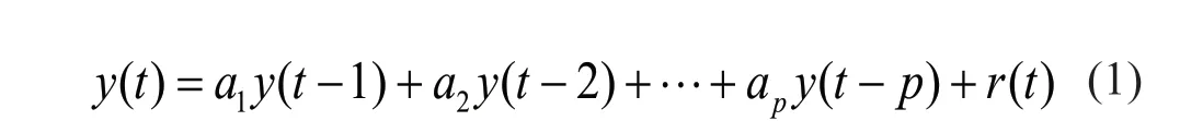
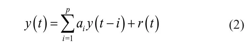
wherey(t) andr(t) are the measured vibration signal and the model residual at timet, which is a Gaussian white noise error with a zero mean. Moreover,a1,a2, …,apdenote the AR coefficients, which can be estimated by one of the parameter estimation techniques (Bisgaard and Kulahci, 2011; Boxet al., 2015), andpis an order of the AR model, which specifies how many unknown parameters should be allocated to the mathematical equation of the model to predict the output data. The other forms of the AR model can be rewritten as:
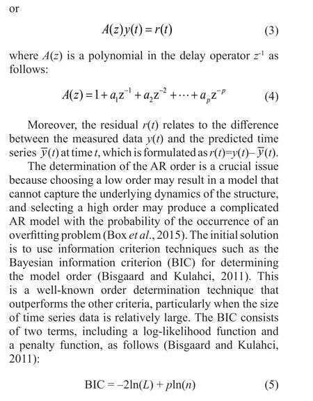
whereLis the maximum likelihood function so that the first term of Eq. (5) can be approximated asnln(σ2),in whichσ2denotes the estimate of the variance of the model residual. Furthermore,nrepresents the number of data points. The process of order determination via the BIC technique and other information criteria is based on choosing a set of relatively large order samples (e.g.,p=1-200), fitting an AR model by using each of the sample orders applied to time series data, and calculating a BIC value. After these procedures, a sample order with a minimum BIC value is determined as the AR model(Entezamiet al., 2019).
3 Proposed feature extraction technique
Feature extraction by time series modeling relies on choosing a time series model and extracting some statistical features of this model (Fassois and Sakellariou,2009). The features extracted from the model should be related to damage; otherwise, even robust feature discrimination algorithms will not provide reasonable or accurate results regarding damage diagnosis. An inaccurate time series modeling may produce improper features with low sensitivity to damage. Therefore,one should attempt to establish an accurate time series representation for response modeling and feature extraction.
As discussed earlier, the important issue in feature extraction via time series analysis is to determine adequate orders of a time series representation so that those enable the model to generate uncorrelated residuals. In other words, the determination of accurate and adequate orders of a time series model guarantees model accuracy(Entezami and Shariatmadar, 2018; Rezaiee-Pajandet al., 2017). Although information criteria such as BIC are capable of determining model orders, appropriate orders of any time series model depend greatly on the property and uncorrelatedness of the residual samples (Boxet al.,2015). In this regard, any time series model that does not satisfy this issue should be improved by choosing better orders. It should be mentioned that since the AR model only requires one order, it is necessary to improve it if the model cannot generate uncorrelated residuals. Under the above-mentioned explanations, the proposed feature extraction method develops an effective algorithm to extract reliable DSFs from the AR model. Figure 1 shows the flowchart and the main steps of this algorithm.As can be seen, it is composed of eight steps that are clarified in the following illustration:
Step 1 - Data acquisition: The step of data acquisition includes choosing the types of excitation, sensors,their locations, and data acquisition devices. This step is followed in the experimental phase and needs good expertise for implementing the dynamic test and the acquisition hardware or software.
Step 2 - Signal pre-processing: Before fitting an AR model to a vibration response, it is important to carry out normalization or standardization processes so as reduce the effect of signal disturbances such as noise. For this purpose, the vibration responses are normalized via the statistical normalization by their mean and standard deviations.
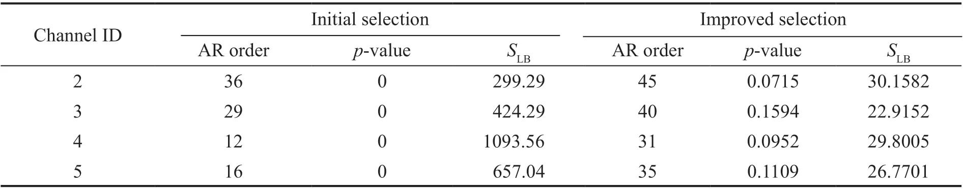
Step 3 - Order determination: In this step, the initial order of the AR model is determined by the BIC, as explained in Section 2.
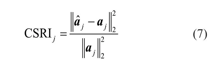
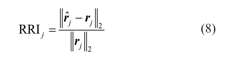
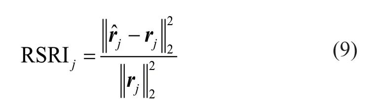
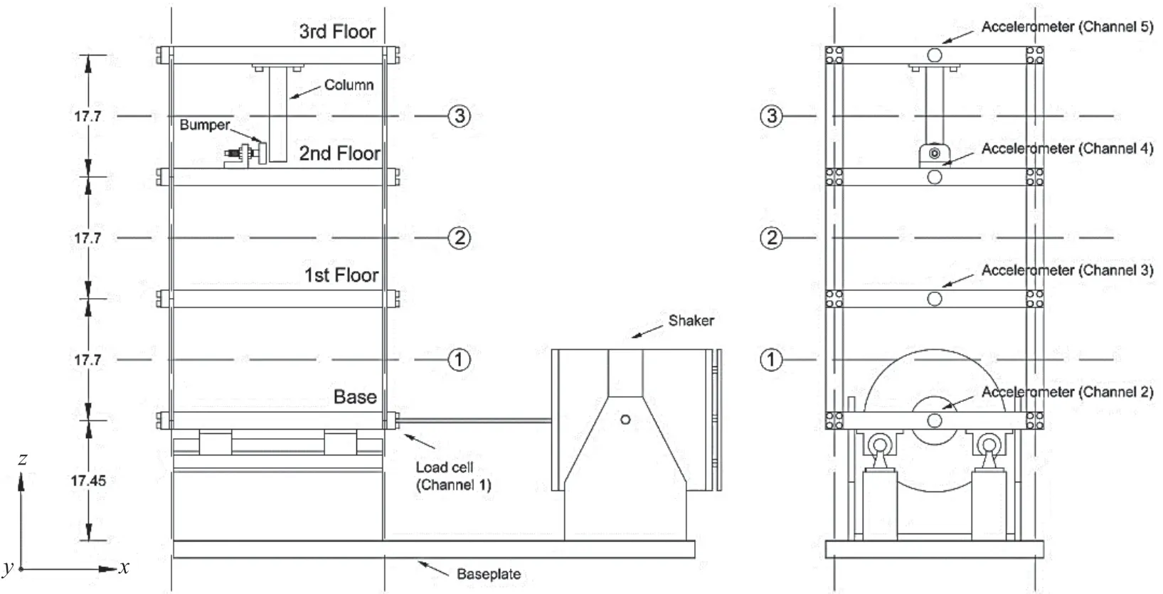
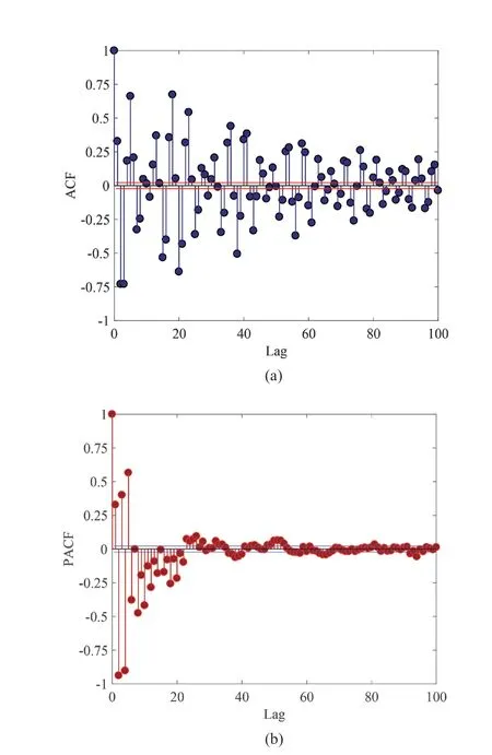
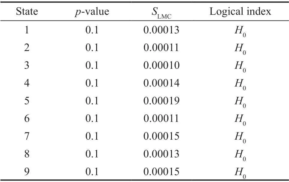
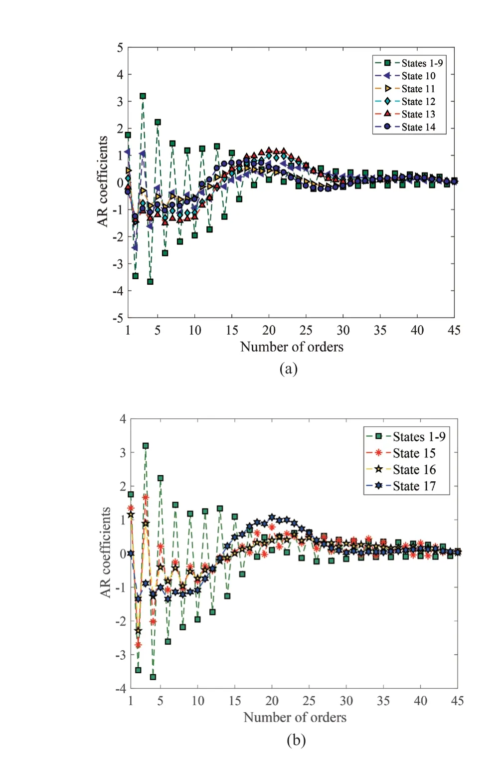
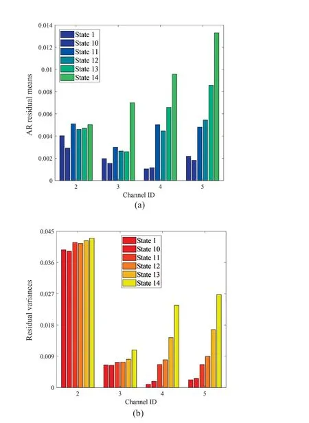
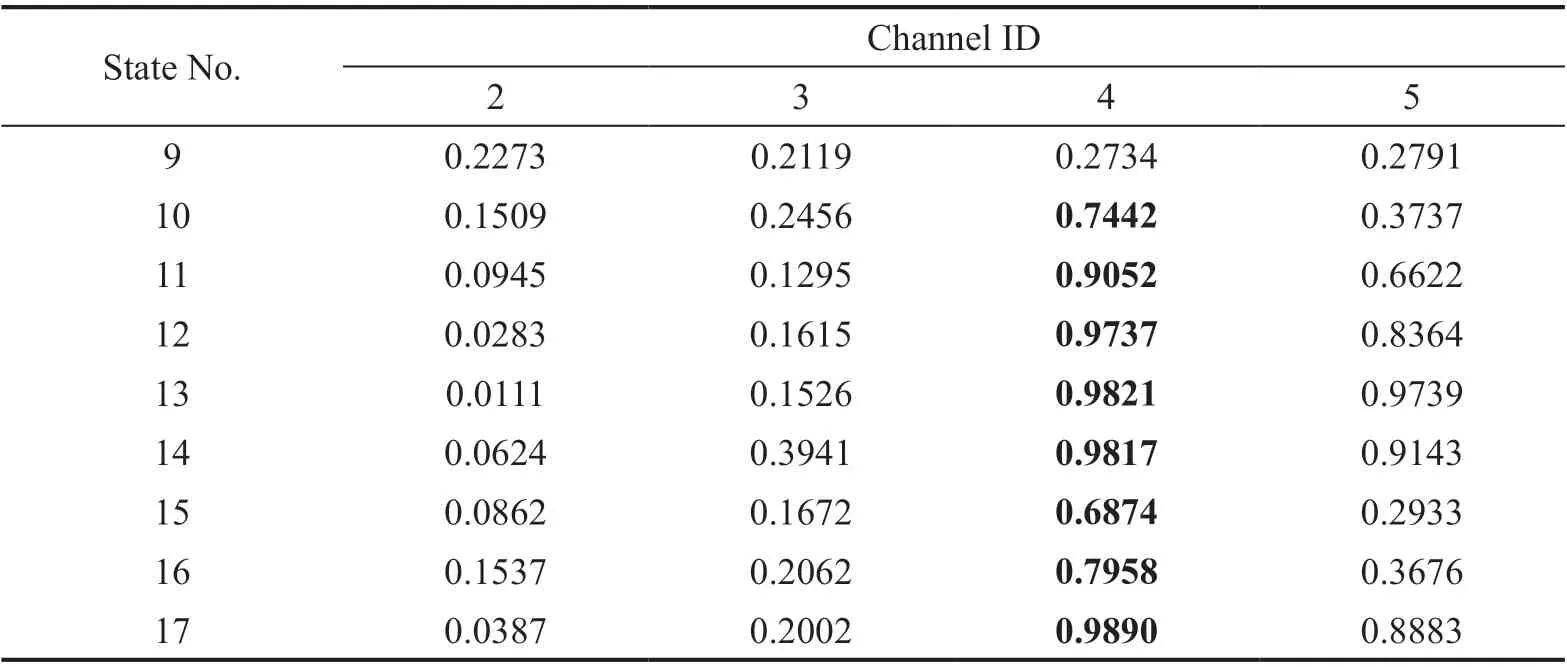
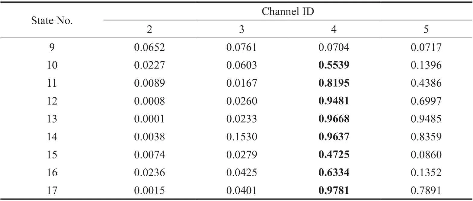
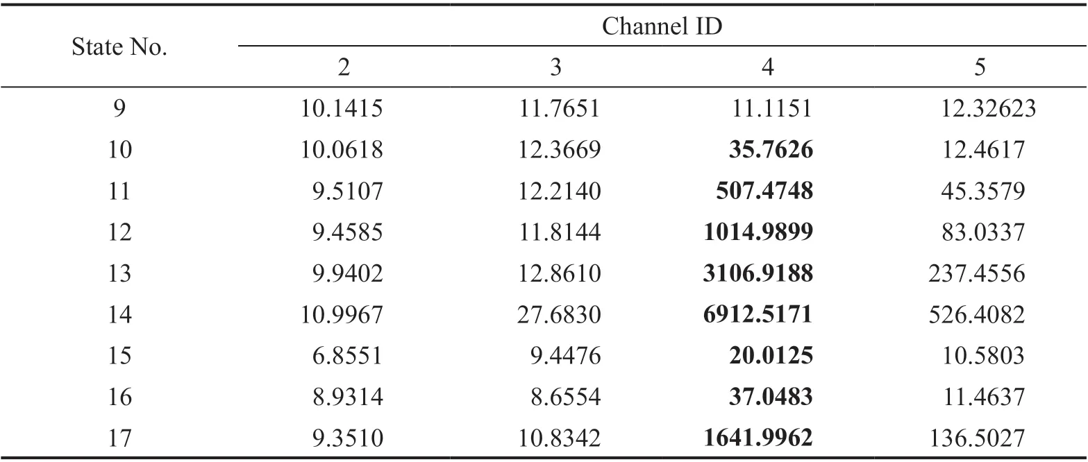
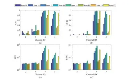
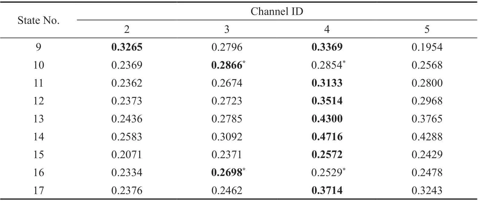
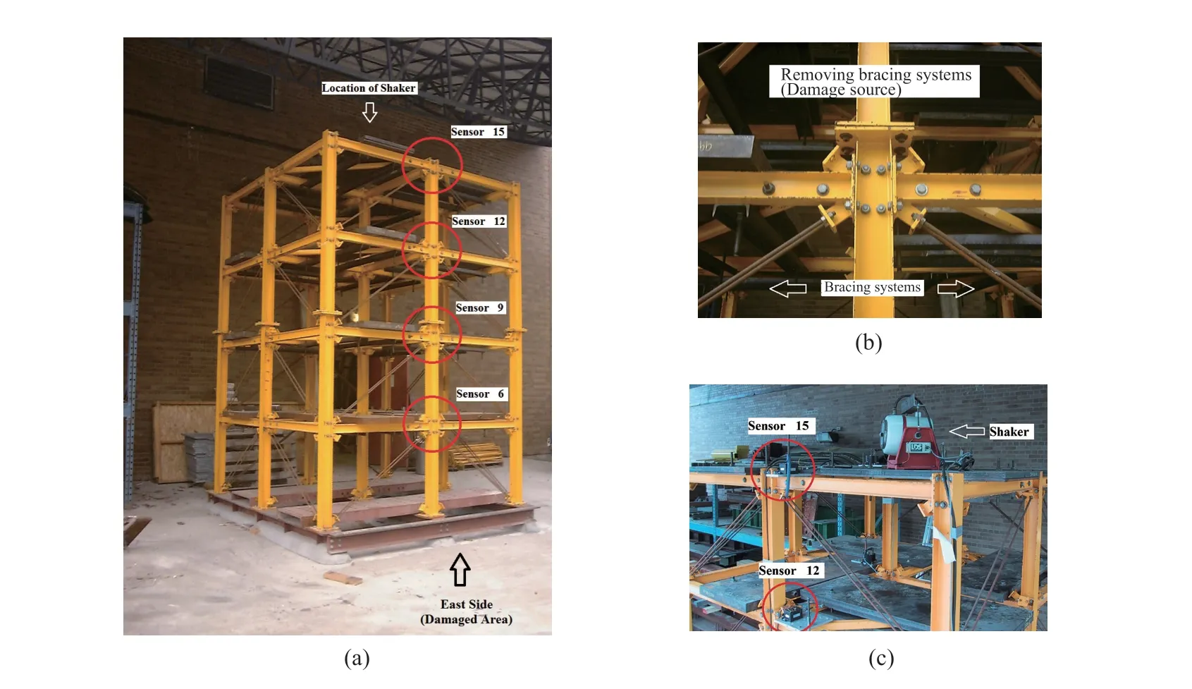
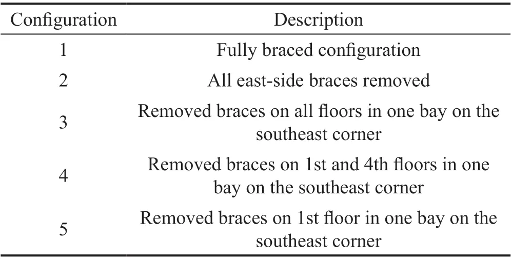
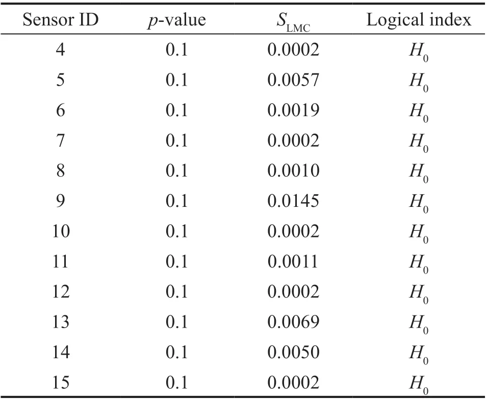
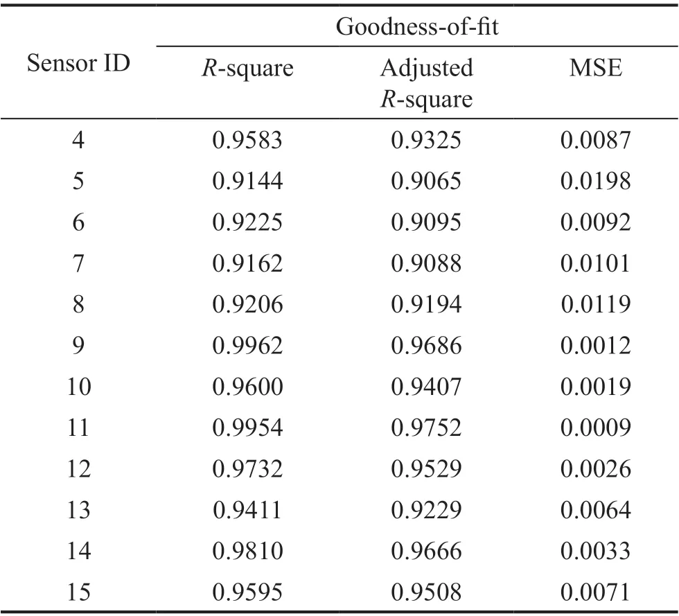
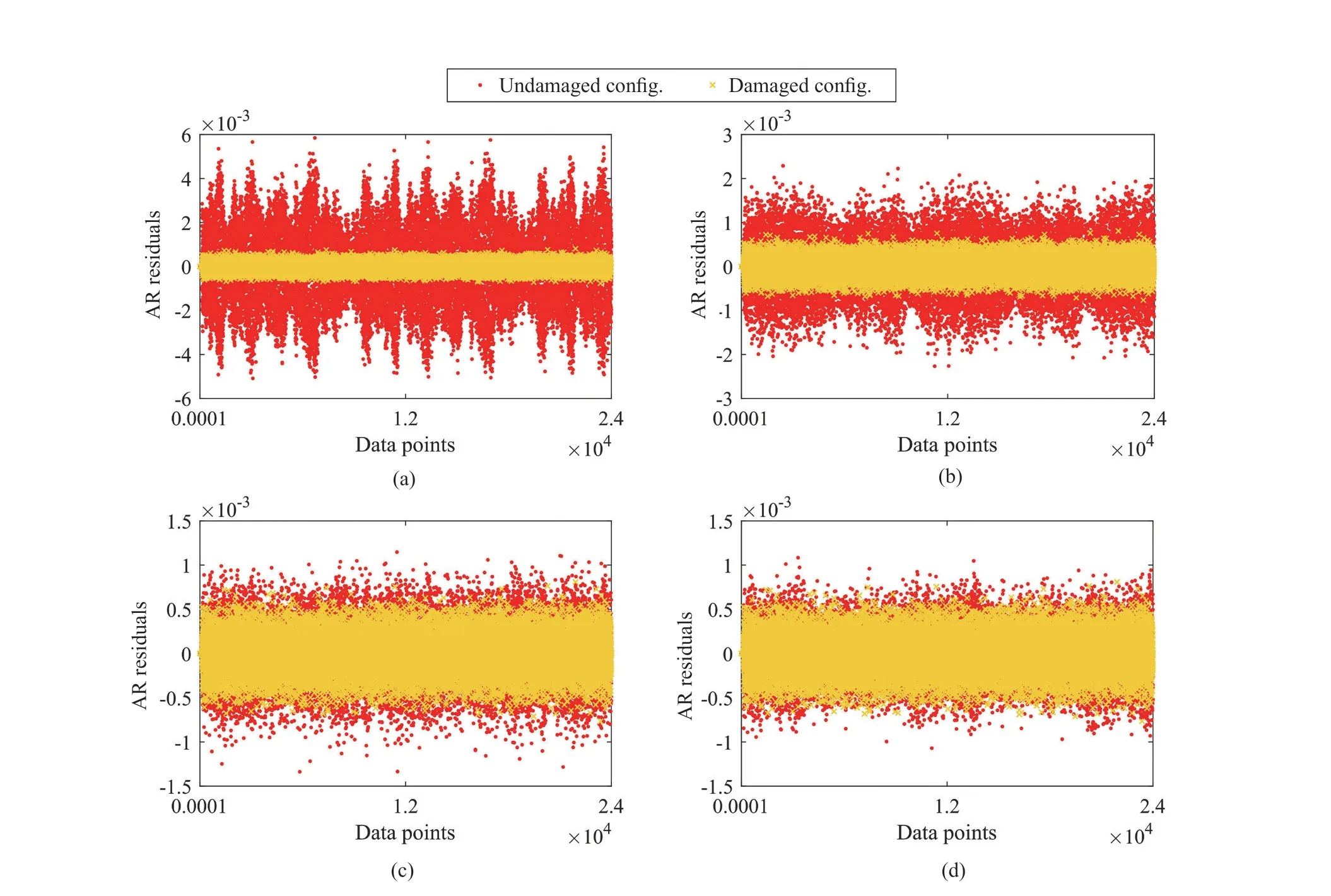
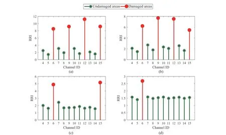
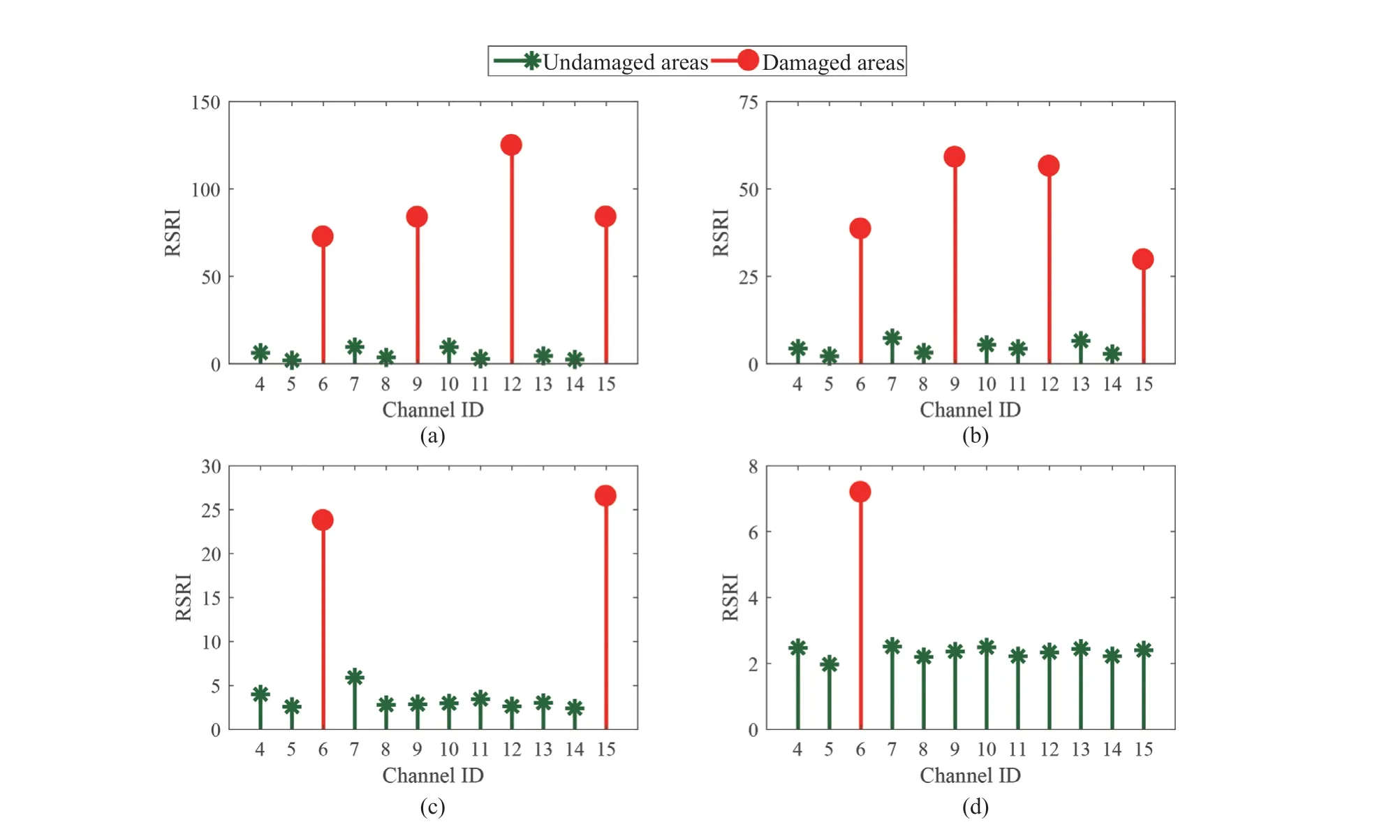
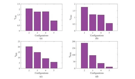
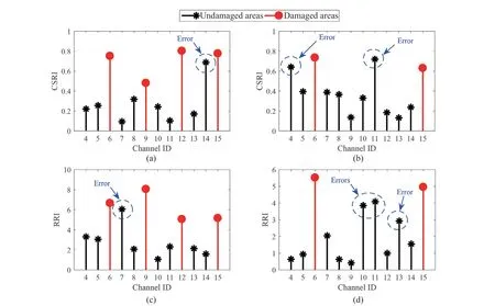
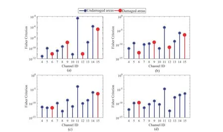
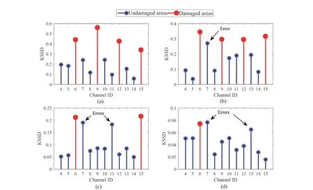
Step 4 - Order improvement: As discussed earlier,although the BIC technique is capable of determining the order of the AR model (and the orders of the other time series models), it is necessary to extract independent or uncorrelated residuals from the fitted time series model. In this step, thus, the initial order of the AR representation gained by the BIC is improved to generate uncorrelated residuals from each model. The criterion for improvement is based on the analysis of the model residuals via the Ljung-Box (LB) hypothesis test (Boxet al., 2015). This test is a tool for evaluating the correlation of residual samples extracted from time series models. Similar to most of the statistical hypothesis tests, it yields some useful outputs such as a probability score orp-value, a critical value orc-value,a test statistic (SLB), and a logical index between the null hypothesisH0and the alternative hypothesisH1. Under a significant levelα, the residual samples of a time series model are uncorrelated, which refers to the null hypothesis or acceptance of the theory or hypothesis, ifp-value>αandSLB Step 5 - Optimal order selection: The use of a unique order from all determined orders is important for extracting the DSFs of the undamaged and damaged conditions of the same size. Moreover, the equality of the size of the DSFs facilitates the process of feature discrimination. In this step, therefore, an optimal order is selected to generalize to all vibration signals on the condition that the residuals of each AR representation are able to produce uncorrelated residuals. Accordingly,the optimal order is the maximum number of the orders obtained from step 4. Step 6 - Parameter estimation: After choosing the optimal order, the coefficients of the AR model are estimated by using one of the current methods such as Yule-Walker, Burg, forward-backward, or least-squares.In this study, the Yule-Walker technique is applied to estimate the AR coefficients. Step 7 - Residual extraction: In this step, the residuals of the AR model for all sensors are extracted by subtracting the measured vibration data from the predicted one that is obtained from the AR representation. Step 8 - DSF extraction: Feature extraction by the AR coefficients relies on fitting the optimal model to the vibration signals of the undamaged and damaged conditions, and estimating the model coefficients regarding both conditions. In contrast, feature extraction by the model residuals is based on fitting an AR model with the optimal order for each vibration response of the undamaged condition, and estimating the model coefficients. Subsequently, this model, along with its details (the optimal order and the estimated coefficients), is applied to predict the vibration response of the damaged state and extract the model residuals in this condition. The idea behind this strategy is that the selected model used in the undamaged condition will no longer accurately predict the responses of the damaged state; therefore, the residual errors related to this condition will increase. Fig. 1 The flowchart and main steps of the proposed feature extraction method using the AR model The supervised learning classifiers are reliant upon the coefficients and residuals of the AR representation extracted from the proposed feature extraction technique. These classifiers fall into the supervised learning class due to the requirement of both the DSFs of the undamaged and damaged conditions for developing a decision-making model for damage localization and quantification. The main idea behind these classifiers is to compute the magnitude of the relative error in the DSFs between the undamaged and damaged conditions.From a mathematical viewpoint, the magnitude of a vector or a matrix can readily be determined by using one of the mathematical norms. The coefficient relative error index (CRI) is one of the coefficient-based classifiers, used on the basis of computing the relative error between the coefficients of the AR representations for each sensor in undamaged and damaged conditions. This classifier is simply formulated as follows: wherej=1, 2, …,srefers to the number of sensors mounted on the structure;aˆjandajare the vectors of the AR coefficients at thejth sensor in the undamaged and damaged conditions, respectively. In this equation,||.||2stands for thel2-norm or Euclidean norm.Considering the CRI values of all sensors, one can derive ans-dimensional vector for these values for damage localization. The advantage of this classifier is that it varies in a range of zero to one, 0 ≤CRI≤ 1, where CRI=0 and CRI=1, and it ideally asserts the undamaged and damaged conditions (areas) of the structure. The coefficient square relative error index (CSRI) is a developed form of CRI, which squares the norms of the numerator and the denominator of CRI for increasing damage detectability and localizability. The equation of CSRI is expressed as follows: Similarly, one can obtain an s-dimensional vector of the CSRI values in which each element represents a value of CSRI at a sensor. The main reason for using CSRI is to achieve more obvious observations for damage localization. The CSRI elements vary from zero to one, so that CSRI=0 declares that the area of a structure did not suffer from damage, while CSRI=1 implies a damaged location. It is worth noting that the vectors of the AR coefficients (â,a) used in Eqs. (6) and(7) containpelements that refer to the optimal order of the AR model. Therefore, this indicates the importance of using the same size of AR coefficients and selecting the optimal order in the proposed feature extraction method. The residual relative error index (RRI) is one of the residual-based classifiers based on computing the relative error between the AR residuals extracted from the proposed feature extraction technique in undamaged and damaged conditions. The formulation of this classifier is similar to the CRI, with a difference in applying the residuals of the AR models rather than the model coefficients. The equation of RRI is given by: whererˆjandrjdenote the vectors of then-dimensional residual samples associated with undamaged and damaged conditions, respectively. Using thel2-norm of relative error in the residual vectors in the denominator and nominator of Eq. (8), a scalar amount of RRI is obtained for each sensor. Therefore, one can obtain ans-dimensional vector of RRI values for damage localization and quantification. Unlike the coefficientbased supervised learning classifiers, the sensor locations with the largest RRI quantities are identified as the damaged areas of the structure. The other type of residual-based supervised learning classifier is the relative square residual index (RSRI),which computes the square RRI to provide better observations in the damage identification process. The formulation of this classifier is similar CSRI, in the following form: The RSRI produces ans-dimensional vector, which represents the value of RSRI for each sensor. Similar to RRI, the sensor locations regarding the largest values of RSRI are identified as the damage locations. The experimental data of a building frame is used to demonstrate the accuracy and effectiveness of the proposed methods. The frame was constructed in a laboratory environment, as shown in Fig. 2. This laboratory model belongs to the Los Alamos National Laboratory, USA (Figueiredoet al., 2009). The acceleration time histories were measured by four accelerometers (the channel 2-5) that were mounted at the centerline of each floor. The sensor signals were sampled at 320 Hz for 25.6 s, which were discretized into 8192 data samples at the time interval of 0.003125 s.An electrodynamics shaker provided a lateral excitation force on the base floor along the centerline of the frame.A center column is suspended from the third floor to simulate a non-linear damage source by using a bumper and an adjustable gap. The acceleration response time histories of all floors and the base are measured under different structural conditions, as described in Table 1. The structural conditions can be divided into four different groups: (1) the baseline condition (state 1),which is an ideal structural state without any damage or uncertainty, (2) the environmental and operational variability (EOV) conditions (states 2-9), (3) the damaged conditions without EOV (states 10-14), and(4) the damaged conditions in addition to the simulated EOV (states 15-17). Fig. 2 The three-story laboratory frame (Figueiredo et al., 2009) Table 1 Structural conditions in the three-story frame (Figueiredo et al., 2009) 5.1.1 Feature extraction Before extracting the AR coefficients and residuals as the DSFs, it is preferable to show the accuracy and adequacy of the AR model and the reasons for the selection of this model in preference to other types of time series models. From a statistical point of view, the autocorrelation function (ACF) and partial autocorrelation function (PACF) are two useful graphical tools for model identification. If the ACF components for a time series response exponentially decrease and the PACF components gradually become zero after a specific lag, it can be argued that the time series response conforms to an AR process (Boxet al., 2015). Figure 3 shows the ACF and PACF plots of the acceleration response data at sensor 4 in the baseline condition. It is obvious from this figure that the components of ACF do not tend to zero and exponentially decrease,whereas the segments of PACF gradually decay to zero approximately after the 30th lag. Fig. 3 The criterion for AR model identification regarding the vibration response at sensor 4 of the first state:(a) ACF, (b) PACF Another investigation for making ensuring the accuracy of choosing the AR model for feature extraction is based on a numerical method. This method is a statistical measure called the Leybourne-McCabe (LMC)hypothesis test, as proposed by Leybourne and McCabe(1994). This statistical test is a measure for checking the stationarity of univariate time series data. In addition,the great merit of this test is its applicability to AR model identification (Daneshvaret al., 2020). Similar to most of the hypothesis tests, it includes some useful outputs,such as ap-value, ac-value, a statistic (SLB), and a logical index betweenH0orH1. Under the significance levelα,if the test accepts the null hypothesis (i.e., the time series data is stationary and conforms to an AR process), the logical index corresponds toH0,p-value>α, andSLMC After choosing the AR model, all of the vibration signals acquired from all sensors are normalized by using the standard statistical normalization method,as mentioned in Section 3. Suppose thatμandσare the mean and standard deviation of each acceleration response data. Hence, the normalized vibration signal is obtained as follows: Table 2 Numerical analysis of the accuracy of choosing the AR model selection by the LMC test wherey(t) andy~(t) are the original and normalized vibration responses, respectively. In the next step, the initial AR orders of sensors 2-5 are determined by the BIC using 150 sample orders. Due to the importance of generating uncorrelated residuals, the initial orders are improved by checking the correlation of the residual samples via the LB hypothesis test. Table 3 presents the numbers of the initial and improved AR orders as well as some outputs of the LB test. As noted in the 4 of the proposed feature extraction technique, the optimal order is the maximum order among the improved AR orders. Hence, the optimal order is identical to 45 and AR(45) and is fitted to the vibrations responses for feature extraction. Since the choice of the maximum number among the improved orders may increase the probability of the overfitting problem, this issue should be checked. Goodness-of-fit statistics such asR-square, adjustedR-square, and mean squared error (MSE) not only provide useful numerical tools for the verification of any time series model, but also it is possible to utilize them to check the underfitting and overfitting problems (Montgomeryet al., 2015).R-square is a number that indicates how the vibration response data fit a time series model. It is the square of the correlation between the time series response and the predicted response values, so that anR-square value equal to 1% or 100% indicates a complete fit and a zero value implies that the model does not fit the data.The adjustedR-square statistic is generally deemed the best indicator of the goodness of fit, in which a value closer to one indicates a better fit. UnlikeR-square, the adjustedR-square can include negative values. In this regard, if the amounts ofR-square and adjustedR-square are similar without any negative value for adjustedR-square, one can conclude that the time series model is neither underfitting nor overfitting (Montgomeryet al., 2015). Furthermore, an MSE value closer to zero is indicative of a fit that is more useful for prediction.Table 4 presents the results of the goodness-of-fit statistics for AR(45) in the first state. It can be seen in this table that theR-square and adjustedR-square values are close to one and together are similar. Moreover, the values of MSE are approximately equal to zero. These conclusions confirm the accuracy and adequacy of time series modeling by AR(45) without any underfitting and overfitting problems. For the AR coefficients as one of the DSFs, AR(45)is fitted to the vibration responses of the undamaged and damaged conditions. Next, the AR coefficients are estimated by using the Yule-Walker approach. For extracting the AR residuals as the other DSFs, AR(45)fitted to the vibration of responses of states 1-9 is applied to predict their vibration responses and to extract the model residuals. The same process is carried out by using AR(45) and the estimated coefficients from the undamaged states. In order to obtain unique coefficients for each sensor, the average of AR coefficients in states 1-9 is computed. Therefore, the optimal order and the average AR coefficients are used to extract the residual samples of the damaged conditions. Figure 4 illustrates the comparisons between the average coefficients of the undamaged states and the damaged conditions. As can be seen, there is an obvious difference in the AR coefficients of the undamaged and damaged conditions,particularly at the initial coefficients. This observation confirms that such damage causes a reduction in the coefficients of the AR models. Additionally, Fig. 5 shows the variations in the mean and variance of the AR residuals of state 1 and states 10-14 in order to investigate the influence of damage on model residuals. Based on the analysis of results, it can be understood that the rate of changes in the statistical properties of the residuals increases by increasing damage severity. It is worth noting that state 14 produces the highest damage level and state 10 is the lowest, as stated in Figueiredoet al. (2009). As a result, it can beconcluded that such damage leads to an increase in the residuals or their statistical properties. Table 3 The initial and improved AR orders Table 4 Goodness-of-fit statistics for AR(45) in the baseline condition It must be mentioned that the computational time for feature extraction of each of the undamaged conditions is roughly equal to 2.8 s and 2.25 s for extracting the AR coefficients and residuals. These procedures for each of the damaged conditions need 1.7 s and 1.4 s. For these processes, a computer with the specifications of IntelTMCore i7-3770, 3.40-3.90 GHz CPU, 16GB RAM has been applied. 5.1.2 Damage localization and quantification Fig. 4 Variations in the AR coefficients at sensor 4: (a) the states 1-9 vs. states 10-14, (b) states 1-9 vs. states 15-17 Once the AR coefficients and residuals have been obtained, they are applied to the proposed supervised learning classifiers for locating and quantifying damage.In order to consider environmental and operational variability, the average of AR coefficients and AR residuals for all channels of states 1-8 are computed to obtain two individual sets of features (i.e., a set regarding the AR coefficients and another associated with the AR residuals) of the previously mentioned undamaged conditions. Moreover, the vibration responses and features of state 9 are considered to be the validation data to examine the accuracy of the proposed classifiers.This means that the vibration responses and features extracted from this state are similarly used as damaged conditions. Since state 9 is undamaged, it is expected that the results of damage localization and quantification of this condition differ from those of states 10-17. Tables 5-8 present the amounts of the proposed classifiers,where the bold value refers to the damage location. As can be seen, the values of the proposed classifiers in state 9 are in the same range and are smaller than the values of classifiers at the damaged location (channel 4).In Table 5 and Table 6, the listed quantities are far from one in the sense that there is no damage in this state;hence, the locations of channels 2-5 are indicative of the undamaged areas. In Table 7 and Table 8, the values of RRI and RSRI of state 9 are roughly the same as the corresponding quantities for channels 2 and 3 of states 10-17. Therefore, the proposed classifiers, with the aid of the DSFs obtained from the proposed feature extraction approach, make accurate decisions for state 9. For states 10-17, it is observed that the classifier amounts at sensor 4 are more than for the other sensors (channels), which means that this area of the frame is the damage location. Fig. 5 The statistical properties of the AR residuals in the damaged conditions: (a) mean, (b) variance More precisely, as the data in Table 5 and Table 6 demonstrate, the amounts of CRI and CSRI of sensor 4 are close to one. From Table 7 and Table 8, the RRI and RSRI values at this channel are larger than the other channels. It should be noted that some classifier quantities at sensor 5 are also considerable. Since the source of damage was mounted between channels 4 and 5, it is reasonable that the mentioned values are large. For the problem of damage quantification, Fig. 6 illustrates the amounts of the proposed supervised learning classifiers in the damaged conditions. For better exhibitions,the logarithmic values of RRI and RSRI are shown.Before analyzing and interpreting the results, it must be explained that structural conditions 10 and 14 produce the lowest and highest levels of damage severity,respectively. Moreover, the severity of damage increases from state 10 to state 14. On the other hand, states 10,15, and 16, as well as states 13 and 17, show the same severities (Figueiredoet al., 2009). With these descriptions, it can be seen in Figs. 6(a)-6(b)that structural conditions 11-14 and 17 at channels 4 and 5 have the CRI and CSRI quantities close to one.Among all of the damaged conditions, state 17 indicates the most severe level of damage (CRI=0.9890 and CSRI=0.9781), and some of the damaged conditions(states 12-14) are approximately in the same level of damage severity. These conclusions reveal that although CRI and CSRI are successful in locating damage and defining damage limits (from 0 to 1), they are not able to provide reasonable results of damage quantification.Nevertheless, there are accurate and more reliable results, as displayed in Figs. 6(c)-6(d), which display the process of damage quantification through the RRI and RSRI classifiers, respectively. It is revealed from these figures that state 14 has the highest level of damage due to a distinct difference with other states at channels 4 and 5. Another conclusion is that the level of damage increases from state 10 to state 14 in ascending order, which reflects the correct results of damage quantification, as reported in Table 1. Furthermore, the quantities of RRI and RSRI do not change at sensors 2 and 3 because they are not the locations of damage.Another note is that the extent of damage at channel 4 is much more than the damage severity present at channel 5. As a consequence, it can be concluded that the residual-based classifiers provide more reliable and precise results of damage quantification compared to the coefficient-based classifiers. Table 5 Damage localization in the laboratory frame via the amounts of CRI Table 6 Damage localization in the laboratory frame via the amounts of CSRI Table 7 Damage localization in the laboratory frame via the amounts of RRI 5.1.3 Comparisons Despite the accurate results of damage localization and quantification via the proposed feature extraction approach and the supervised learning classifiers, itis necessary to compare them with some existing techniques. On this basis, some comparative analyses are implemented here. The first comparison is concerned with the effect of using initial orders obtained from the BIC technique on the extracted features and the results of damage localization and quantification. According to Table 3, AR(36) is fitted to all vibration responses to extract the model coefficients and residuals. In this comparison, the outputs of CSRI and RRI in some structural states of the laboratory frame are considered,as listed in Table 9. Accordingly, it can be seen that the quantities of CSRI and RRI regarding state 9 are listed separately in the same range and the previously mentioned classifiers in states 14 and 17 precisely identify the location of the damage at sensor 4. Despite having larger values of CSRI and RRI at sensor 4, which are associated with states 10 and 16 compared to the other sensors, some unreliable results are also available:they are marked by the symbol “*”. This is because the amounts of CSRI and RRI at sensors 2 and 3 are close to sensor 4, and are larger than the corresponding values at sensor 5. Therefore, one can conclude that the improvement of the initial orders leads to extracting better DSFs. Table 8 Damage localization in the laboratory frame via the amounts of RSRI Fig. 6 The process of damage quantification by the proposed supervised learning classifiers in the damaged conditions: (a) CRI,(b) CSRI, (c) RRI, (d) RSRI The other analysis is related to the comparison of the proposed classifiers with the Fisher criterion (Mosaviet al., 2012), using the AR coefficients and Kolmogorov-Smirnov statistical distance (KSSD) (Royet al., 2015)through the AR residuals. It must be clarified that such features are those that have been applied to locate damage via the proposed classifiers, as mentioned in the preceding section. Table 10 and Table 11 present the values of the Fisher criterion and KSSD for damage localization, respectively, where the bold quantities indicate the damage locations and the amounts with the symbol “*” are representative of errors in damage localization. From Table 10, one can realize that the Fisher criterion fails in locating damage due to its poor performance for the localization of channel 4 as the damaged area of the laboratory frame. Although channel 5 was placed in the vicinity of the bumper (the source of damage), channel 4 shouldbe identified as the main damage location. In Table 11,however, it is seen that KSSD outperforms the Fisher criterion, and this statistical distance could identify the location of channel 4 as the damaged area in states 11-15 and 17. Nonetheless, it is not able to provide precise results of damage localization in states 10 and 16.Therefore, the results of comparative analyses confirm that the proposed supervised learning classifiers are superior to the classical indices. Table 9 Damage localization in the laboratory frame based on the initial order Table 10 Damage localization in the laboratory frame by use of the Fisher criterion (×10-6)and AR coefficients For further investigation, the ASCE benchmark structure in the second phase (Dykeet al., 2003) is considered to validate the accuracy and effectiveness of the proposed methods. This scale model structure was located at the Earthquake Engineering Research Laboratory at the University of British Columbia (UBC)in Canada. It was mounted on a concrete slab outside of the structural testing laboratory on the UBC campus to simulate typical ambient vibration conditions. The ASCE structure included 2-bay × 2-bay steel frames in four stories, with sizes of 3.6 m tall and 2.5 m × 2.5 m in the plan. Figure 7(a) shows a general view of this structure. The members were constructed of hot-rolled, grade 300W steel (nominal yield stress 300 MPa). The sections were specifically designed for this scale model test framework. The columns and floor beams were B100×9 and S75×11 sections, respectively.In each bay, the bracing systems, as shown in Fig. 7(b),included two ½-inch diameter steel rods placed parallel along the diagonal. To make mass distribution reasonably realistic, a one-floor slab was placed in each bay per floor.Fifteen accelerometers, including FBA and EPI sensors with specifications of a 0-50 Hz frequency range and a sensitivity of 5 V/g, were mounted on the east, west sides and the center portion of the structure (Entezami and Shariatmadar, 2018) to measure acceleration timehistories. Three accelerometers were installed at ground level, and their acceleration time histories were not considered in this article due to poor dynamic behavior and information (Entezami and Shariatmadar, 2018;Sarmadiet al., 2020a). Table 11 Damage localization in the laboratory frame by KSSD and AR residuals Fig. 7 (a) The ASCE benchmark structure and locations of some the sensors at the damaged area (the east side), (b) the bracing systems and the damage source, (c) the excitation source by a shaker Table 12 The undamaged and damaged configurations of the ASCE structure (Dyke et al., 2003) Table 13 Numerical analysis of the accuracy of the AR model selection by the LMC test There were three types of excitation sources including an impact hammer; a shaker; and ambient vibration caused by wind, pedestrians, and traffic in the vicinity of the structure. In this article the vibration responses stemming from the shaker are utilized. Figure 7(c)illustrates the shaker and some visible sensors. To create different damage scenarios, the structure was subjected to different levels of damage, as listed and described in Table 12. The source of the damage shown in these configurations was meant to remove the bracing systems on the east side. 5.2.1 Feature extraction The first step in feature extraction is to confirm the accuracy of choosing the AR model for response modeling. For this purpose, Table 13 presents the outputs of the LMC hypothesis test for the vibration responses of configuration 1 at the 5% significance level. As can be seen, allp-values are larger than 0.05 and all test statistics are smaller than thec-value, which is identical to 0.1460, leading to the logical indexH0. Therefore, it can be inferred that the selection of the AR model for feature extraction is reasonable. On the other hand, Table 14 lists the initial and improved orders obtained from the proposed feature extraction approach and the outputs of the LB hypothesis test. In this table, one can see that the use of the improved orders enables AR models to generate uncorrelated residuals since allp-values are larger than 0.05 and all quantities ofSLBare smaller than thec-value, which corresponds to 31.4104 under the 5% significance level for the LB test. According to the proposed feature extraction approach, finally, AR(128)is fitted to all vibration responses to extract the model coefficients and residuals. In order to ensure the lack of occurrence of the overfitting problem due to using AR(128), Table 15 gives the amounts ofR-square, adjustedR-square, and MSE regarding all sensors in the first configuration.Based on the descriptions in the previous experimental study, one can observe in this table that theR-square and adjustedR-square values are approximately close to one,respectively, without any negative values for adjustedR-square. Additionally, the values of MSE roughly correspond to zero. Therefore, it can be concluded that the use of AR(128) does not lead to the overfitting problem and it provides a good fit for response modeling. Using the selected optimal order, the model coefficients of the undamaged and damaged configurations are estimated by using the Yule-Walker technique. Figure 8 shows the variations in the AR coefficients at sensor 6 for all configurations to investigate the influence of damage on these features. It should be noted that the damage location at the vicinity of sensor 6 is common to all damaged configurations.Hence, the AR coefficients of this sensor are considered in this comparison. From Fig. 8 it can be seen that most of the variations are associated with configurations 2 and 3. Since the level of damage severity in configuration 4 is smaller than in configurations 2 and 3, one can observe that the rate of variations shown in Fig. 8(c) is smaller than the corresponding variations displayed in Figs. 8(a)-8(b). Finally, the smallest variations in the AR coefficients relate to configuration 5, which includes the lowest level of damage severity. These conclusions confirm the sensitivity of the AR coefficients, as obtained from the proposed feature extraction approach to damage. The other comparison is related to the AR residuals at sensor 6. In this regard, Fig. 9 compares the variations in the residual samples of AR(128) between the undamaged and damaged configurations. As can be seen,regarding the occurrence of damage in configurations 2 and 3, by considering their severity levels, this leads to considerable increases in the residual data points so that the increases regarding the second configurationare larger than for the other one. The increases are also observable in Figs. 9(c)-9(d), but those are not as clear as the corresponding increases shown in Figs. 9(a)-9(b).These results also prove the sensitivity of the AR residuals that are extracted from the proposed approach to damage. Table 14 The initial and optimal AR orders in configuration 1 Table 15 Goodness-of-fit statistics for AR(128) in configuration 1 It is worth mentioning that the computational time for extracting the AR coefficients and residuals of the configuration 1 are equal to 136 s and 117 s. For each of the remaining configurations, the computational time roughly corresponds to 108 s and 100 s for the extraction of the model coefficients and residuals. It must be added that these procedures have been performed by a computer with the specifications of IntelTMCore i7-3770, 3.40-3.90 GHz CPU, 16GB RAM. 5.2.2 Damage localization and quantification Using the AR coefficients and residuals regarding the undamaged (configuration 1) and damaged(configurations 2-5) states, Figs. 10-13 illustrate the results of damage lo=calization by using the proposed supervised learning classifiers CRI, CSRI, RRI, and RSRI, respectively. Since the east side of the ASCE structure was simulated as the damaged area, it is expected that the mentioned classifiers would be able to identify the locations of sensors 6, 9, 12, 15 in configurations 2 and 3; sensors 6 and 15 regarding configuration 4; and sensor 6 in configuration 5 as the damaged areas of the structure. From Figs. 10(a)-10(b), it can be seen that the proposed classifier CRI succeeds in precisely locating the damaged areas associated with the second and third configurations. Although this classifier is also capable of identifying the damage locations of the remaining configurations, there are some errors in the results.In other words, one can observe in Figs. 10(c)-10(d)that the locations of sensors 11 and 10 are mistakenly identified as the damaged areas. In the following section,it can be seen that the other proposed classifiers are able to locate the damaged areas in all configurations without any error. Therefore, one can conclude that the proposed classifiers CSRI, RRI, and RSRI, except for CRI in the minor damage scenarios, accurately succeed in locating damage. Fig. 8 Comparison of the AR coefficients between the undamaged and damaged configurations at sensor 6: (a) configurations 1 and 2, (b) configurations 1 and 3, (c) configurations 1 and 4, (d) configurations 1 and 5 Fig. 9 Comparison of the AR residuals between the undamaged and damaged configurations at sensor 6: (a) configurations 1 and 2, (b) configurations 1 and 3, (c) configurations 1 and 4, (d) configurations 1 and 5 Fig. 10 Damage localization in the ASCE structure by CRI: (a) configuration 2, (b) configuration 3, (c) configuration 4,(d) configuration 5 Fig. 11 Damage localization in the ASCE structure by CSRI: (a) configuration 2, (b) configuration 3, (c) configuration 4,(d) configuration 5 The other investigation is related to damage quantification. For this problem, thel2-norm of the CRI, CSRI, RRI, and RSRI values for all sensors are computed to provide numerical scores in quantifying the severity of damage rather than applying the direct classifier amounts at specific sensor locations. The results of damage quantification in the ASCE structure are shown in Fig. 14, whereηCRI,ηCSRI,ηRRI, andηRSRIstand for thel2-norms of the classifiers CRI, CSRI,RRI, RSRI, respectively. As can be seen, the residualbased classifiers RRI and RSRI can quantitatively estimate the levels of damage severities so that theirl2-norms are gradually reduced from configuration 2 to configuration 5. Nevertheless, the coefficient-based classifiers CRI and CSRI cannot provide reasonable results of damage quantification because thel2-norms of CRI and CSRI in the fourth configuration are either larger than the third one or roughly equal to it. Fig. 12 Damage localization in the ASCE structure by RRI: (a) configuration 2, (b) configuration 3, (c) configuration 4,(d) configuration 5 Fig. 13 Damage localization in the ASCE structure by RSRI: (a) configuration 2, (b) configuration 3, (c) configuration 4,(d) configuration 5 5.2.3 Comparisons This section presents some comparative analyses for indicating the superiority of the proposed methods to some existing techniques. The first comparison is concerned with the influences of the initial and optimal(improved) orders on the process of damage localization.In this regard, Fig. 15 shows the results of damage localization in the second and fourth configurations by the CSRI and RRI classifiers, using the coefficients and residuals of AR(114), in which the order number 114 is the maximum quantity of all initial orders obtained from using the BIC technique. Despite the capability and effectiveness of the proposed classifiers CSRI and RRI in locating damage, one can see that the use of the optimal number of the initial order cannot provide reliable features that cause inaccurate damage localization, with some errors. The second comparison relates to the evaluation of the performances of the coefficient-based classifiers.Accordingly Fig. 16 shows the results of damage localization in the ASCE structure by the use of the Fisher criterion and the AR coefficients obtained from the proposed feature extraction approach. As expected,this classifier is not able to localize either the multiple or the single damage scenarios due to serious errors in the process of damage localization. In Figs. 16(a)-16(b),the locations of sensors 6, 9, 12, 15 should be identified as the damaged areas. Moreover, one should identify sensors 6 and 15 in Fig. 16(c) and sensor 6 in Fig. 16(d)as the main damaged areas of the ASCE structure. Thus,the comparison between the CRI and CSRI classifiers proposed in this article, using the Fisher criterion, reveals that the proposed classifiers are superior to the Fisher criterion, even CRI, and this criterion is not sufficiently reliable for damage localization. Fig. 14 Damagequantification of the ASCE structure using the l2-norm of the values of the proposed classifiers: (a) CRI, (b) CSRI,(c) RRI,(d)RSRI Fig. 15 Damage localization in the ASCE structure using AR(114) for feature extraction: (a) configuration 2 by CSRI,(b) configuration 4 by CSRI, (c) configuration 2 by RRI, (d) configuration 4 by RRI Fig. 16 Damage localization in the ASCE structure according to the Fisher criterion, using the AR coefficients: (a) configuration 2,(b) configuration 3, (c) configuration 4, (d) configuration 5 Fig. 17 Damage localization in the ASCE structure by KSSD using the AR residuals: (a) configuration 2, (b) configuration 3,(c) configuration 4, (d) configuration 5 The final comparative analysis is based on comparing the performances of the residual-based classifiers.On this basis, the results of damage localization in the ASCE structure by KSSD and AR residuals and presented in Fig. 17 intend to compare this statistical distance with the proposed RRI and RSRI classifiers.As can be seen, KSSD is successful in identifying the damaged areas of the ASCE structure at the locations of the above-mentioned sensors, particularly as displayed in Fig. 17(a). However, there are some errors in locating damage related to configurations 3-5, as can be observed in Figs. 17(b)-17(d). Therefore, one can conclude that the proposed classifiers RRI and RSRI are superior to KSSD in locating damage and providing better results than in this statistical distance without any error. In this study, new supervised learning classifiers were proposed to locate and quantify single and multiple damage cases by time-series features extracted from a new feature extraction technique based on AR modeling.In this technique, the residuals and coefficients of the AR representation for each sensor were utilized as the main DSFs in the supervised learning classifiers. These classifiers were based on computing thel2-norm of the relative error in the DSFs of the undamaged and damaged conditions. Two types of classifiers (CRI and RRI) were formulated as the direct relative errors, based on the coefficients and residuals of the AR models. The other classifiers (CSRI and RSRI) were based on using the square relative errors of these features. The experimental datasets of a laboratory frame and the ASCE structure were utilized to verify the robustness and performance of the proposed techniques, along with comparative analyses. In conclusion, the results of this study suggest that the features extracted from the proposed feature extraction method are sensitive to damage, so that the coefficients of the AR model tend to be decreased during the occurrence of damage. In addition, the AR residuals,along with their statistical characteristics, such as mean and variance, increased due to the occurring structural damage. Regarding the process of damage localization by the coefficient-based classifiers, sensor locations close to one were identified as the damage locations.In contrast, based on the residual-based classifiers,the sensor locations associated with the maximum amounts of the residual-based classifiers indicated the damaged areas of the structure. In most cases, the proposed classifiers were successful in locating damage,but the sole classifier CRI made some errors in minor damage scenarios related to the ASCE structure. For the problem of damage quantification, it was seen that the coefficient-based classifiers were not effective due to some erroneous results. In contrast, the residualbased classifiers gave clearer and better results of damage quantification compared to the coefficient-based classifiers. The comparative analyses indicate that the proposed supervised learning classifiers, even CRI, are superior to the conventional Fisher criterion and KSSD.Moreover, it was seen that the optimal order obtained from the improved orders enables the AR model to extract better features than the optimal order from the initial orders gained by the conventional BIC technique. Acknowledgement The authors would like to express their sincere gratitude to the IASC-ASCE Structural Health Monitoring Task Group and the Engineering Institute at the Los Alamos National Laboratory for being able to access their experimental datasets.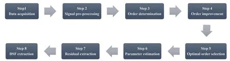
4 Supervised learning classifiers
4.1 Coefficient relative error index

4.2 Coefficient square relative error index
4.3 Residual relative error index
4.4 Residual square relative error index
5 Experimental studies
5.1 The laboratory frame


5.2 The ASCE structure


6 Concluding remarks
杂志排行

Earthquake Engineering and Engineering Vibration的其它文章
- A review of the research and application of deep learning-based computer vision in structural damage detection
- Experimental study of vertical and batter pile groups in saturated sand using a centrifuge shaking table
- Analytical evaluation and experimental validation on dynamic rocking behavior for shallow foundation considering structural response
- Effect of geofoam as cover material in cut and cover tunnels on the seismic response of ground surface
- Dynamic response of concrete face rockfill dam affected by polarity reversal of near-fault earthquake
- Analyzing uncertainties involved in estimating collapse risk with and without considering uncertainty probability distribution parameters