Analyzing uncertainties involved in estimating collapse risk with and without considering uncertainty probability distribution parameters

Mohammad Amin Bayari, Naser Shabakhty and Esmaeel Izadi Zaman Abadi

1. Department of Civil Engineering, Najafabad Branch, Islamic Azad University, Najafabad 8514143131, Iran

2. School of Civil Engineering, Iran University of Science and Technology, Tehran 16844, Iran

Abstract: In the present study, modified Ibarra, Medina and Krawinkler moment-rotation parameters are used for modeling the uncertainties in concrete moment frame structures. Correlations of model parameters in a component and between two structural components were considered to analyze these uncertainties. In the first step, the structural collapse responses were obtained by producing 281 samples for the uncertainties using the Latin hypercube sampling (LHS) method,considering the probability distribution of the uncertainties and performing incremental dynamic analyses. In the second step,281 new samples were produced for the uncertainties by the central composite design (CCD) method without considering the probability distribution of the uncertainties and calculating the structural collapse responses. Then, using the response surface method (RSM) and artificial neural network (ANN) for the two simulation modes, structural collapse responses were predicted. The results indicated that the collapse responses at levels of 0 to 100% obtained from the two simulations have a high correlation coefficient of 98%. This suggests that random variables can be simulated without considering the probability distribution of uncertainties, by performing uncertainty analysis to determine structural collapse responses.Keywords: uncertainty analysis; collapse response; artificial neural network; response surface method

1 Introduction

Sideway collapse, which is defined as a lateral instability of a structure due to strong ground motions,has been considered by researchers in recent years (Lielet al., 2009; Zareian and Krawinkler, 2007; Zareianet al., 2010). In this regard, identifying different uncertainty resources to predict collapse capacity and accurately describe the seismic performance of structures is of great importance (Ugurhanet al.,2014). Two main uncertainty resources affect the collapse probability of structures;i.e., aleatory uncertainties resulting from the inherent nature of phenomena and epistemic uncertainties due to the lack of knowledge and inaccurate analytical models.In determining structural collapse probabilities, intensive motion features such as ground motion duration,earthquake frequency content, and earthquake intensity parameters are considered as aleatory uncertainties(record to record), while the assumptions made in the structural analysis are treated as epistemic uncertainties.Epistemic uncertainties can be reduced by developing scientific relations, collecting more data, and using a proper analytical model (Der Kiureghian and Ditlevsen,2009). Due to the relatively limited knowledge of model parameters and collapse-related behavior,modeling uncertainties have received much attention in simulating the structural collapse response. They are needed to idealize nonlinear deformation demands and various sources of degradation both at the component and structure levels. Concentrated plastic hinge models are the best candidate for modeling structural collapse responses. Parameters employed to define concentrated plastic hinge models are typically calibrated by empirical relationships, which are a major source of uncertainties for structural collapse response simulation (Ugurhanet al., 2014).

The incremental dynamic analysis (IDA) is introduced to consider the intrinsic variability effects of an earthquake in the seismic response analyses of structures. In this method, an earthquake record is scaled to cover a wide range of seismic intensities to consider uncertainties in seismic intensity prediction.Furthermore, to consider existing uncertainties in the frequency contents and spectral shapes of earthquakes,a considerable number of earthquake records are employed. This method is considered to predict the capacities of structures in the FEMA-350 Code (FEMA,2000).

Simulation methods such as the Monte Carlo and the Latin hypercube sampling (LHS) are used to incorporate these uncertainties. A large number of simulations are required to cover the probability distribution of uncertainties, which is a time-consuming practice. To reduce computational efforts, the response surface method (RSM) is proposed in combination with simulation methods. In addition to RSM, alternative methods can be employed to consider uncertainties in prediction models, including artificial neural network(ANN) and neuro-fuzzy network (Beheshti-Avalet al.,2015).

Vamvatsikos and Cornell (2004), Zareian and Krawinkler (2007) studied IDA-based methods to evaluate structural collapse. Ibarra and Krawinkler(2005) proposed a method to evaluate the global collapse of structures based on the relative intensity measure and engineering demand parameter. They defined global collapse as the inability of a structural system to resist gravity loads in the presence of seismic effects. The relative intensity increases until the system response becomes unstable; that is, the relative intensityengineering demand parameter curve becomes flat.They named the largest relative intensity as the collapse capacity. Haseltonet al.(2008) tested reinforced concrete columns to calibrate and determine the proper measures of the tri-linear model parameters proposed by Ibarraet al. (2005). Then, they proposed a set of empirical relationships for each parameter by conducting statistical studies and multivariate regression analysis. Lignos and Krawinkler (2010) proposed a database for modeling steel components based on the tri-linear model of Ibarraet al. (2005). Li (1996) demonstrated that any form of functions and its derivatives can be estimated using ANN, while the use of ANN creates lower prediction errors than RSM. Gomes and Miguel (2004) compared RSM and ANN in evaluating the reliability of a structure that had an implicit limit state function. They indicated that the use of these two methods to estimate the limit state function decreases the reliability of the evaluation when compared to the Monte Carlo method.

Bucher and Most (2008) compared response function methods and indicated that selecting the response function would be different depending on the problem.According to the examples of this study, response surface methods based on polynomial functions, radial basis functions (RBFs), and ANN have the ability to accurately consider failure conditions. Burattiet al.(2010) employed a parabolic model to estimate the structural response of a reinforced concrete moment frame considering uncertainties in structural features and ground motion parameters when an earthquake happens. They drew fragility curves according to the evaluated parabolic model. Park and Towashiraporn(2014) applied RMS for the probability evaluation and seismic vulnerability of steel bridges. They fitted the limit state function in the form of a second-order polynomial function by considering the uncertainties involved and not considering the interaction terms,calculating the probability of exceeding the damage states based on the fitted response surface functions.Khojastehfaret al.(2014) employed ANN and RSM in combination with the Monte Carlo method to develop collapse fragility curves by considering uncertainties in a steel moment frame. They showed that it is more accurate to determine the mean measures and standard deviations of the fragility curves by the ANN-based Monte Carlo simulation approach than by the RSMbased Monte Carlo method. Borekciet al.(2014)studied the collapse potential of SDOF systems caused by dynamic instability with stiffness and strength degradation. They introduced an equation to estimate the collapse period of SDOF systems as a function of the strength reduction factor, ductility level, and post-capping stiffness ratio. Investigating structural reliability requires a long computation time. In this regard, Gholizadeh and Mohammadi (2016) employed a wavelet back-propagation (WBP) neural network (NN)to predict the required deterministic and probabilistic structural nonlinear seismic responses at performance levels. Karimi and Şensoy (2016) used metaheuristic algorithms to evaluate the collapse responses of steel moment frames by considering different uncertainty sources. They adopted the IDA method to incorporate record-to-record uncertainties. The model uncertainties were applied by backbone curves and hysteresis loops.Also, cognitive uncertainties were provided at three levels of material quality. The analytical questions of the RSM were derived from the IDA results obtained using the Cuckoo algorithm, which predicts the means and standard deviations of collapse fragility curves. The Takagi-Sugeno-Kang model was employed to represent the material quality. Finally, collapse fragility curves with the uncertainties were obtained by various material quality values derived from the fuzzy Takagi-Sugeno-Kang model. The results indicated that better risk management strategies in countries with weak material quality control create cognitive uncertainties in fragility curves and the mean annual frequency. Zhanget al.(2017) introduced a novel approach, i.e., time-dependent reliability analysis with response surface (TRARS), to estimate the timedependent reliability for nondeterministic structures under stochastic loads. They treated random variables and the maximum responses of uncertain structures as the input and output parameters, respectively. They also proposed a novel iterative procedure by introducing the response surface (RS) model. Moreover, they used a Butcher strategy to produce initial sample points while employing the gradient projection technique to produce new sample points to update the RS model in each iteration. Then, the time-dependent reliability indices and probabilities of failure were obtained using the firstorder reliability method over a certain design lifetime.Karimi and Beheshti Aval (2018) applied adaptive neuro fuzzy inference system (ANFIS) models based on grid partition (GP), subtractive clustering (SC), and fuzzy C-means (FCM) to analyze uncertainties and predict seismic fragility curves of a steel moment frame. They indicated that ANFIS-FCM predicts fragility curves more accurately than GP and SC methods. Gholizadeh and Aligholizadeh (2019) proposed a meta-model to reduce the computation burden of the Monte Carlo method in the optimization setting. The computation burden of a reliability-based optimal seismic design (RBOSD) is very high due to the huge number of nonlinear pushover analyses. To cope with this problem, they used a simple multilayer perceptron (MLP) model as an NN model to predict the necessary deterministic and probabilistic seismic responses during optimization. A meta-model composed of WPB was introduced for evaluating seismic responses. According to the FEMA-P695 Code (FEMA,2009), the total system collapse uncertainties (βTOT) are calculated by combining different uncertainty sources,including record-to-record (βRTR), design requirements(βDR), test data (βTD), and modeling (βMDL). Fattahi and Gholizadeh (2019), Hassanzadeh and Gholizadeh(2019) employed such uncertainties to determine the collapse margin ratio (CMR) for optimal structures,graphing the optimal structures′ fragility curves. Palanci(2019) introduced a risk assessment model for one-story precast industrial structures by fuzzy logic. Karimi and Şensoy (2020) adopted the optimized fuzzy method FCM-PSO to determine collapse fragility curves by considering the uncertainties. They revealed that this method is advantageous with regard to both accuracy and execution time in estimating the mean and standard deviation of fragility curves. In this study, the input,output, and relations of the fuzzy-based risk assessment model were determined by the reference buildings. The supervised learning method was used to determine the membership function of fuzzy sets and found that fuzzy logic is a promising technique for seismic assessment of structures and can be used as an effective instrument in rapid performance screening of the structures.

In the present study, two different methods of producing random samples and simulation with and without considering the probability distribution parameters of the uncertainties are employed to investigate the effects of uncertainties on structural collapse responses. The LHS method was used to generate samples with considering the probability distribution of the uncertainties, while the central composite design (CCD) was adopted to produce samples without considering the probability distribution of the uncertainties. Moreover, a combination of the above-mentioned simulation methods, RSM, and ANN was employed to predict risk and collapse fragility curves.

2 Model estimation and prediction methods

2.1 Artificial neural network (ANN)

Artificial neural network (ANN) is a method used to estimate functions and predict different systems.Such networks yield acceptable results when there are nonlinear relationships between the input and output of a system. Any network is made up of an input layer, an output layer, and one or more hidden layers. There are a number of neurons inside each of the layers that are connected by weighted connections (Fig. 1). During the network training, the weighs are continuously adjusted to minimize errors. To transfer the outputs of each layer to the next layers, purline, tansing, tangent hyperbolic and sigmoid functions are typically used.

An ANN structure is the multi-layer perceptron(MLP). An MLP can be trained using nonlinear functions such that it can estimate and predict any measurable function. Using a set of real input and output data, ANNs employ training algorithms to form hidden connections between input and output data through weight coefficients,biases, and the applied functions of each layer′s outputs.A portion of data (70%, for example) is typically used to train the network and the remaining portion is employed in data validation and network prediction tests.Various training algorithms have been employed to train ANNs,one of the most important of which being error back propagation algorithm (Anderson, 1995).

2.2 Response surface method (RSM)

In this study, the CCD is used to design the model. CCD includes a full factorial design or twostage fractional factorial design with axial and central points. Using such designs, the curve of a system can be estimated. The design is performed based on three levels of factorial points, axial points, and central points,(Fig. 2).

The number of experiments in CCD is calculated as Eq. (1)

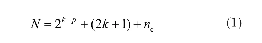
whereNis the number of experiments,kis the number of variables,pis a fraction of full factorial design, andncis the number of replications. The three terms in Eq. (1) denote factorial points, star points (including axial and central points), and the number of replications,respectively. Figure 3 shows CCD for three factors.

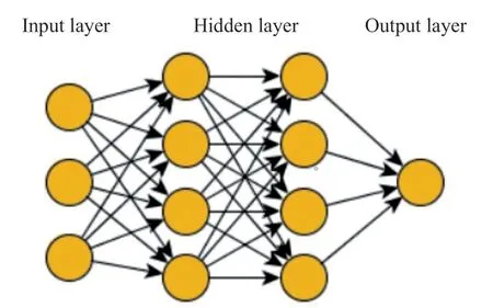
Fig. 1 Structure of a multi-layered perceptron (MLP)

Fig. 2 Factorial, central, and axial points in CCD

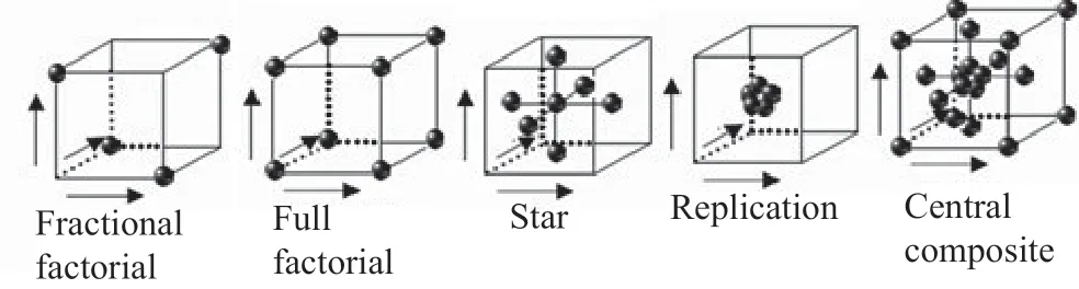
Fig. 3 CCD for three factors

CCD provides a quadratic equation as Eq. (2)

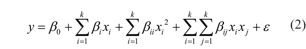
whereβ0,βi,βiiandβijare the constant, linear, quadratic,and interaction coefficients of the factors, respectively.xiandxjare independent coded variables. Equation (2) is a polynomial regression model. The unknown polynomial coefficients are calculated by minimizing the sum of squares of residuals (i.e., the difference between the observed values and estimated function values) (Myerset al., 2009).

3 Structural dynamic analysis

3.1 Dynamic analysis of structure

Incremental dynamic analysis (IDA) is a method to determine the fragility curves of structures′ limit states under different seismic intensities. To perform IDA, proper parameters must be selected to reflect the intensity measure (IM) and demand measure (DM).A proper IM selection leads to lower dispersion in the structure′s response to various earthquakes and thus more accurate estimation of the responses′ statistical measures. In the present study, IM was considered to be the spectral acceleration in the fundamental period of the structure (Sa(T1)). DM is a parameter selected to make the best structural response reflection, which was considered to be the maximum inter-story drift in this study; i.e., maximum among the floors and during the total earthquake time. For IDA analysis, earthquake records were selected and each record was scaled to a small measure of IM that produced linear behavior in the structure′s model, under which time history analysis became nonlinear. The process of scaling IM continues on a proper algorithm until the structural collapse limit is obtained. For the incremental trend of IDA, it is required to select IM values using a proper algorithm to optimize the number of analysis points such that the minimum number of points in the initial linear areas and the maximum number of points in the collapse-prone areas are selected to achieve sufficient accuracy. As a result, the distances between consecutive IMs for each earthquake record can be determined in proportion to its collapse level. The algorithm used in this study for IDA was adapted from the Hunt-Fill algorithm (Vamvatsikos and Cornell, 2002).

After completing each IDA stage, the IM variations were plotted versus the DM of the record.

3.2 Structural collapse criteria

From an engineering perspective, collapse occurs when the lateral drifts of one or more floors becomes larger than the other floors such that the structural system is no longer able to resist the gravity loads due to the secondary moment induced by the building′s weight (P-Delta effect). Thus, according to FEMA-350 Code (FEMA, 2000), IDA can be employed to estimate the structural collapse capacity. According to the code′s recommendation, the collapse point is considered to be equal to the occurrence of one of the following:

- Numerical non-convergence in the structural analysis algorithm;

- A slope of 20% of the initial elastic slope in the IDA curve; and

- Maximum inter-story drift exceeding 0.1.

It was observed in many cases that the determination of structural collapse based on the non-convergence criterion or the minimum slope contradicts real observations and engineering experience in terms ofθmaxcreated in the structure. To handle this problem,structural collapse is simultaneously controlled by two criteria of minimum slope and 0.1 ≤θmax.

According to the earthquake intensity method,collapse limit state refers to an intensity of earthquake that collapses the structure. In other words, IMcapor IMcollapserepresents the last point of seismic intensity on the IDA curve under which the structure does not collapse. After IMcap, the IDA curve slope falls below 20% of the elastic slope or the inter-story drift exceeds 0.1.

For each IDA curve, there is a point with a seismic intensity corresponding to collapse that is denoted by IMcollaps. The possible curve of fitting the mentioned points on several IDA curves represent collapse fragility curves, which are defined as Eq. (3) (Tothong and Cornell, 2007):

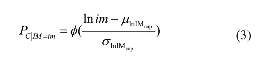
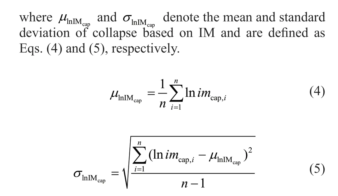
whereimcap,iis the IMcapvalue of recordi, andnis the number of records.

3.3 Probabilistic seismic demand analysis (PSDA)

Probabilistic seismic demand analysis (PSDA) is a good method to calculate the mean annual frequency(MAF) of exceedance of various given values.

PSDA integrates the site-specific seismic hazard curve (e.g., spectral acceleration hazard curve) calculated by probabilistic seismic hazard analysis (PSHA) with the nonlinear dynamic analysis results of the structure collected using a set of accelerograms.

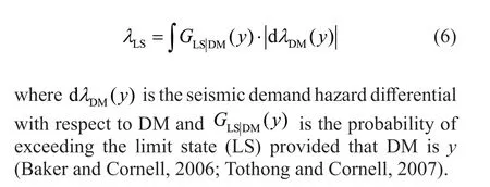
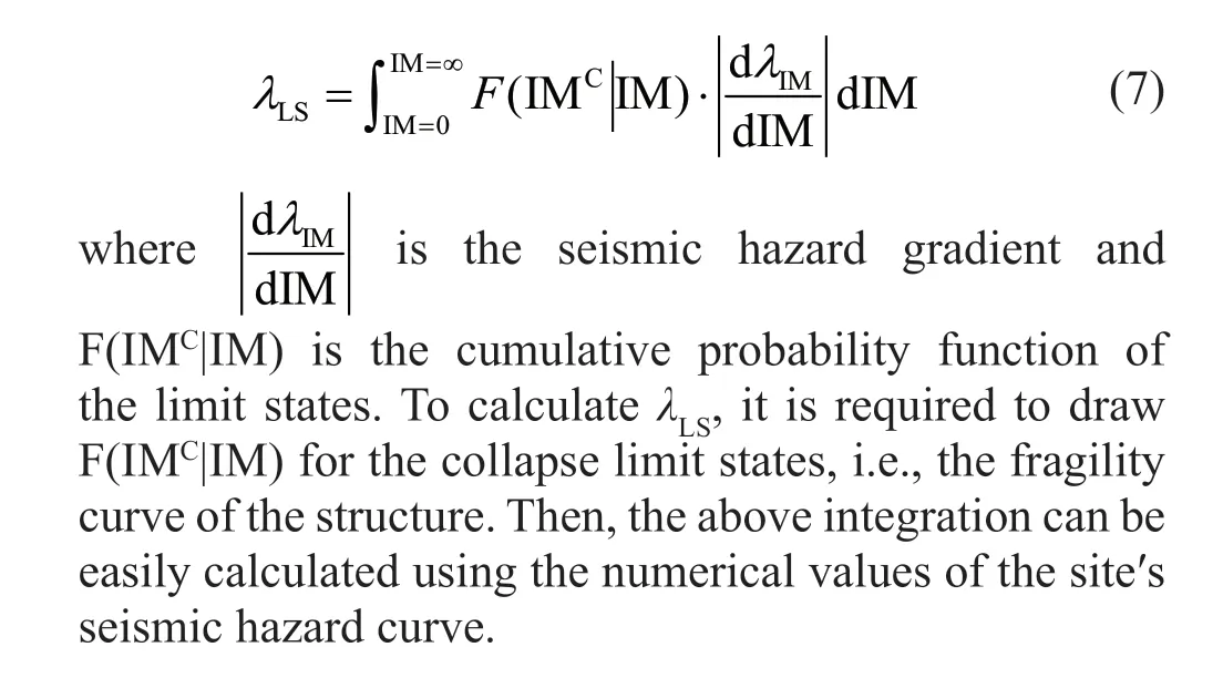
The mean annual frequency (MAF) of exceedance of a given limit state, i.e.,λLS, is calculated as Eq. (6)

4 Modeling

4.1 Structural model

A four-floor structure with a concrete moment frame system was employed in this study. Figure 4 depicts the structure′s plan. The structure is symmetric in plan and elevation. Thus, nonlinear analyses can be performed on the structure on one of the lateral resisting frames,applying the P-Delta effects of the entire structure to the selected moment frame. The structural system selected to resist against the lateral loads is the perimeter moment frame. The lateral resisting systems in thex-direction of the plan are frames 1 and 5. The drifts of the entire structure in this direction are withstood by these two perimeter frames. Therefore, the other internal frames of the structure (known as the space frames or gravity frames) are only under the gravity loads. For the perimeter frames that resist lateral loads of the structure,the gravity loads that are directly withstood by the perimeter frames are different from the loads induced by the P-Delta effects. To consider the P-Delta effects,a pinned-end rigid column without lateral stiffness,known as the leaning column, is employed. The column is connected to the main structure by rigid beams (Fig. 5).To obtain the most accurate results in calculating structural collapse, the nonlinear concentrated plastic hinge model was used. Moreover, OpenSees software was employed for modeling and the nonlinear dynamic analyses. The pushover curve of a four-story frame with ID 1008 proposed by Haseltonet al.(2008) was used to verify the model. Figure 6 shows the pushover curve of the modeled structure and the frame with ID 1008.

A total of 22 pairs of the far-fault records (a total of 44 records) proposed by FEMA-P695 (FEMA, 2009)were used for the IDA.

Fig. 4 Plan of the structure

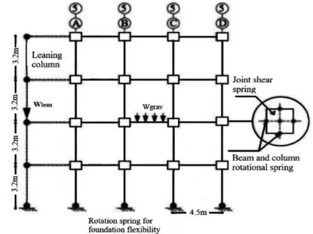
Fig. 5 Two-dimensional analytical moment frame model

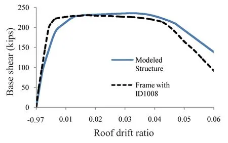
Fig. 6 Comparing the pushover curve of the modeled structure and the frame with ID 1008

4.2 Moment-rotation parameters of concentrated plastic hinge model

4.3 IDA surves of structure

Incremental dynamic analysis (IDA) curves of the structure along with their 16th, 50th, and 84th percentiles are shown in Fig. 8.

4.4 Mean annual frequency of collapse limit state

The mean annual frequency (MAF) of the collapse limit state is calculated by extending Eq. (7) as

4.5 Seismic hazard curve

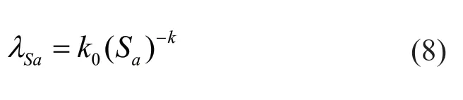
To calculate the seismic hazard gradient, the seismic hazard analysis of the site is required. Analyzing the seismic hazard for a site yields a uniform hazard spectrum with the return period of 475 years and 2,475 years. Then, the spectral accelerations of the return period of 475 and 2,475 years can be obtained for the site according to the fundamental period of the structure.The annual frequency of exceedance of the seismic intensity (i.e., the spectral acceleration in this study) is typically estimated by a linear relation in the logarithmic space as Eq. (8)whereλSais the reverse earthquake return period andSais the spectral acceleration corresponding to the uniform hazard spectrum at the return periods of 475 and 2,475 years. Moreover,kis the seismic hazard curve slope at the intended capacity andk0is the shape coefficient of the seismic hazard curve. To evaluate the seismic demand probability of the model, a site that was only affected by a point source and having the following properties was selected:

- Earthquake return period is 200 years;

- Magnitude of the event is 7.2;

- Nearest distance from the fault is 11 km;

-Vs30is 360 m/s for the site′s soil;

- Reverse type fault; and

- First mode period of the structure is 0.96.

The uniform hazard spectrum of the site at the return period of 475 years and 2,475 years is shown in Fig. 9.

Once the uniform hazard spectrum and fragility curves of the structure are obtained, the mean annual frequency of limit states can be calculated using Eq. (7).The mean annual frequencies of the collapse limit states are provided in Table 1.

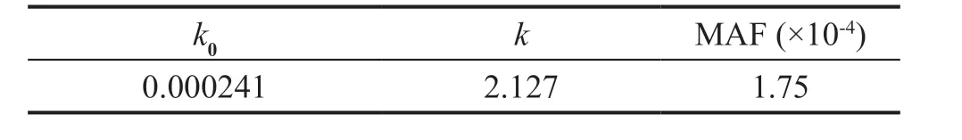
Table 1 Seismic hazard parameters and mean annual frequency of collapse limit states

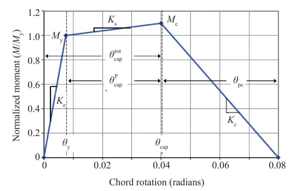
Fig. 7 Tri-linear backbone curve of the plastic hinge model

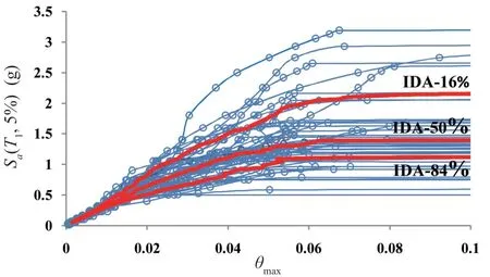
Fig. 8 IDA curves of the structure

5 Uncertainty analysis

5.1 Uncertainties

The concentrated plasticity model parameters introduced in Section 4.2 are considered as epistemic uncertainties. The mean values of the parameters are calculated using the equations proposed by Haseltonet al.(2008). The parameters and their logarithmic standard deviations are as follows (Haseltonet al., 2008;Haselton and Deierlein, 2008):

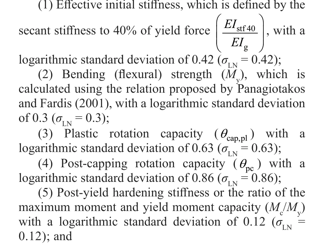
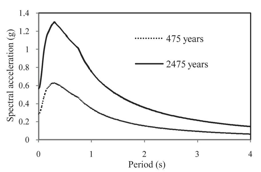
Fig. 9 Uniform hazard spectrum of the site at hazard level of 475 and 2,475 years

(6) Energy dissipation capacity for cyclic stiffness and strength deterioration (λ) with a logarithmic standard deviation of 0.64 (σLN= 0.64).

Six rotation-moment parameters of the concentrated plastic hinges were considered as epistemic uncertainties for the beam and column components - i.e., a total of 12 epistemic uncertainties (six for the beam and six for the column).

To evaluate the correlation of the model parameters in a component and between two structural components,the database built by Haseltonet al.(2008) was employed. The correlation coefficients provided in Table 2 (Ugurhanet al., 2014) were used to define correlations between the parameters of a structural component and correlation between the parameters of two structural components.

To incorporate the existing uncertainties in predicting the seismic intensity, an earthquake record is scaled such that it covers a wide range of intensities. Moreover, an acceptable number of earthquake records are used to consider the uncertainties in the frequency content and spectrum shape of earthquakes.

5.2 Sampling, simulation and satistical data production methods

Table 2 Correlationsbetween parameters of a component and two structural components

According to Eq. (9) and the Cholesky decomposition method, dependent multivariate random variables are produced in the following steps:

1. Produce a lower triangular matrix of the correlation matrix or covariance matrix using the Cholesky method;

2. Produce independent random variables with a mean of 0 and a standard deviation of 1;

3. Use Eq. (9) to produce dependent random variables; and

4. Repeat steps 1 to 3 to generate the intended number of variables.

It is required to produce and simulate a sufficient number of samples for uncertainties to predict collapse fragility curves by considering epistemic uncertainties using RSM and ANN for the 12 introduced uncertainties(six belonging to the plastic hinge parameters of beams and six to the plastic hinge parameters of columns).

In this study, using the CCD method at a factorial level of 1/16, 281 samples were produced and simulated for the 12 epistemic uncertainties. The CCD samples were independent with a uniform distribution, the mean of 0,and the standard deviation of 1. To compare the results obtained from the CCD samples, 281 new independent samples were produced for the 12 uncertainties using the LHS method with considering the probability distribution of the uncertainties. The LHS independent samples also had a mean of 0 and a standard deviation of 1.

Z1is a 281 × 12 matrix of the LHS independent normal variables produced with considering uncertainties probability distribution.Z2is a 281 × 12 matrix of the CCD samples generated without considering uncertainties probability distribution. Hence, Eq. (11)is applied to produce dependent multivariate random variables as Eq. (10)

where ～Lis the lower triangular matrix corresponding to the covariance matrix obtained using the Cholesky decomposition.

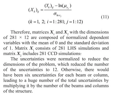
To extend Eq. (10) to other beams and columns, the normalized matrix of the dependent random variables is generated using Eq. (11)

6 Model outputs

6.1 Results of IDA analysis for different simulations

MatricesX1andX2were built using the normalized dependent variables to determine the input variables to perform nonlinear dynamic analyses on the 12 uncertainties of the structure (Eq. (11)). Then, to obtain the structural collapse responses, IDA was performed on each uncertainties simulation according to matricesX1andX2using the 44 introduced records and Hunt-Fill algorithm. Therefore, the mean collapse capacity (μSaorμlnSa), collapse standard deviation (σlnSa), and mean annual frequency (MAF) of collapse were obtained for each simulation.

Figure 10 represents the methodology of the present study to predict structural collapse responses by the RSM and ANN, with and without considering the probability distribution parameters of the uncertainties.

For both LHS and CCD methods, corresponding collapse responses were obtained and compared at statistical levels of 0 to 100%.

Fig. 10 Flowchart of the proposed methodology

Fig. 11 Correlation coefficient between μSa values at levels of 0 to 100% obtained from LHS and CCD methods

Therefore, according to Figs. 11 to 14, the correlation coefficients between the collapse responses at statistical levels 0 to 100% for the LHS and CCD methods are 0.99562, 0.99426, 0.99261, and 0.97955 forμSa,μlnSa,σlnSa, and MAF, respectively.

Fig. 12 Correlation coefficient between μlnSa values at levels of 0 to 100% obtained from LHS and CCD methods

Given the correlation coefficient (R) of above 0.98 between the collapse responses at the statistical levels of 0 to 100% for the two simulation methods,it was concluded that the CCD method can be used to produce samples and analyze uncertainties without considering the probability distribution parameters of the uncertainties.

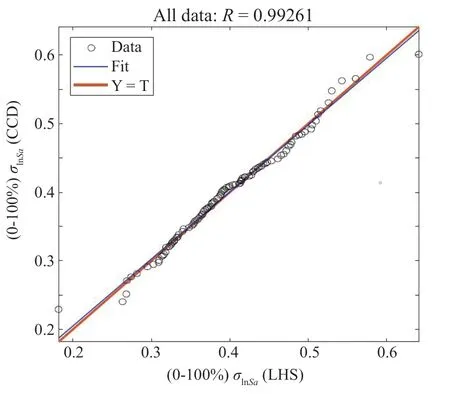
Fig. 13 Correlation coefficient between σlnSa values at levels of 0 to 100% obtained from LHS and CCD methods

6.2 Comparing different prediction methods

In this study, ANN and RSM were employed to predict collapse risk and collapse fragility curves by considering model uncertainties. The data of the input layer for 12 uncertainties consisted of 281 normalized independent variables generated by the LHS method (Z1)and 281 normalized independent variables generated by the CCD method (Z2). The target data were mean collapse capacity (μSaorμlnSa), collapse standard deviation (σlnSa),and mean annual frequency (MAF) obtained from IDA for the simulations. On the other hand, the output data in the ANN output layer were the predicted mean collapse capacity, collapse standard deviation, and mean annual frequency. To assess and compare the accuracy of the prediction methods, three criteria were employed: 1)correlation coefficient (R), 2) mean square error (MSE),and 3) root mean square error (RMSE), which are defined as Eqs. (12), (13) and (14), respectively. Moreover, the estimation error was calculated using Eq. (15):

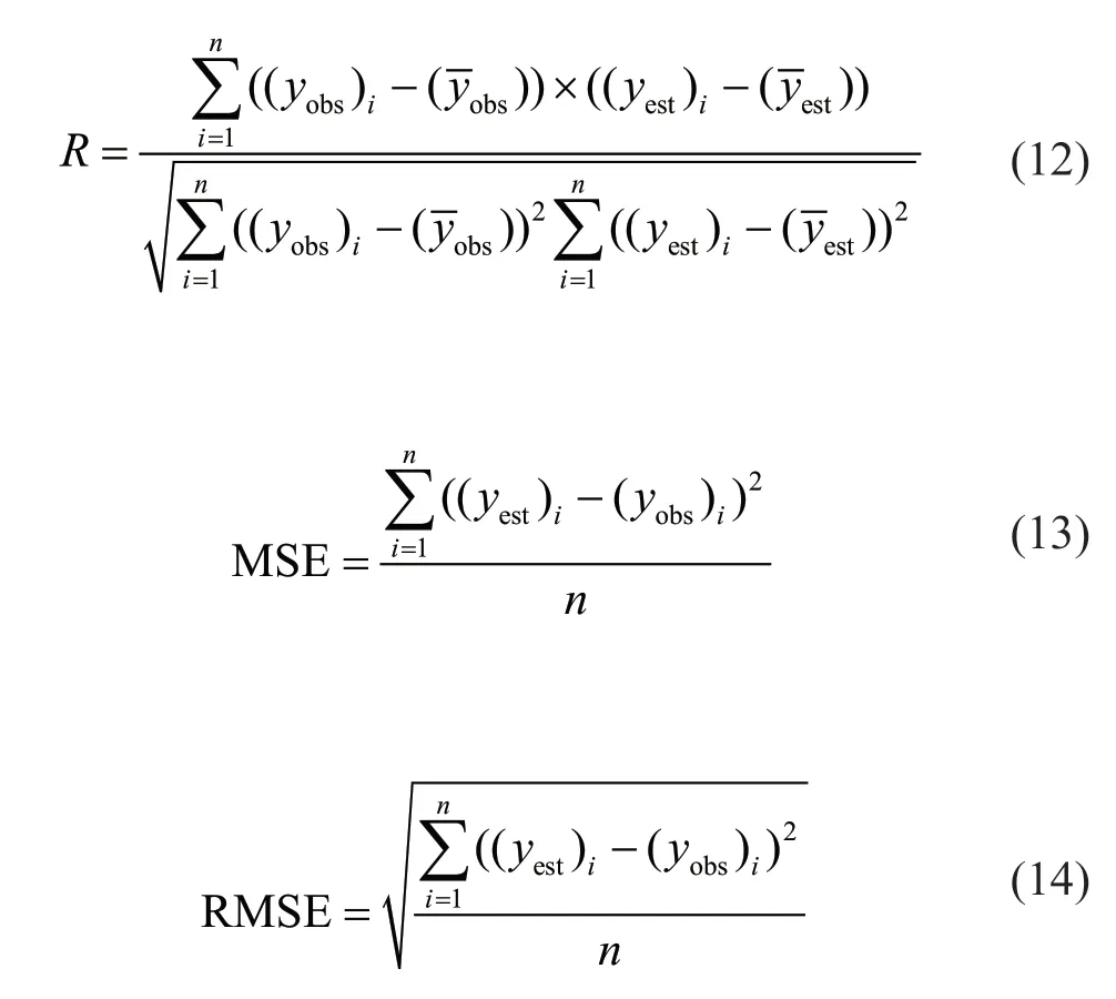
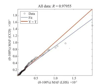
Fig. 14 Correlation coefficient between MAF values at levels of 0 to 100% obtained from LHS and CCD methods

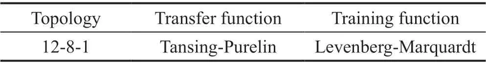
Table 3 ANN structure

The Tansig and Purline transfer functions were used in the hidden and output layers, respectively. The ANN was a feed-forward network with a back-propagation algorithm. Also, the Levenberg-Marquardt (LM)algorithm was applied to train the network. In this study,70% of the data were used as training data, while the remaining 30% were employed as the test data.

Tables 4 and 5 provide the correlation coefficients(R) between the target data and the output data along with MSE and RMSE values for 281 LHS simulations and 281 CCD simulations for the training data, test data,and all data by the ANN.

Additionally, Table 6 represents the correlation coefficients (R) between the target data and the output data along with MSE and RMSE values for 281 LHS simulations and 281 CCD simulations for the all data by the RSM.

Three different tests were performed to compare the prediction methods to the IDA results for both LHS and CCD simulations. In the first step, structural collapse responses were calculated by different methods while all the uncertainties were set to their mean values (Table 7).Then, collapse fragility curves were drawn (Fig. 15). It is seen in Fig. 16 that the maximum errors ofμSa,μlnSaandσlnSaunder RSM and ANN for the LHS method are about 6% and errors of MAF under RSM and ANN are 9% and 6%, respectively. At the same time, for CCD method, the maximum errors ofμSa,μlnSaandσlnSaunder RSM and ANN are about 6%, while the error ofMAFunder RSM and ANN is about 6%.

In the second step,Savalues corresponding to the collapse probability at the levels of 16%, 50%, and 84% were calculated (Table 8). The maximum error under RSM and ANN for the LHS and CCD methods is approximately 3.5%.

In the third test, structural collapse responses of LHS and CCD methods at levels of 16%, 50%, and 84% areprovided in Tables 9 and 10 for IDA, RSM, and ANN results.

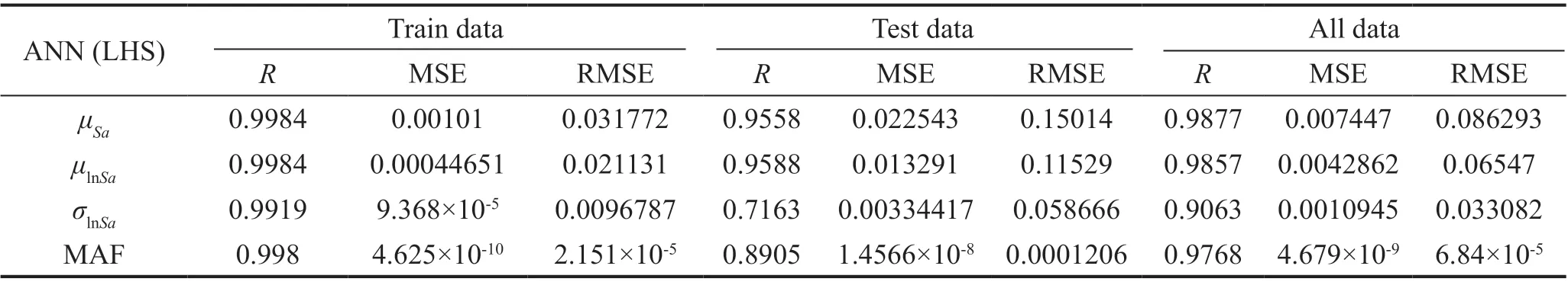
Table 4 Correlation coefficients (R), MSE, and RMSE of responses predicted by the ANN (LHS)

Table 5 Correlation coefficients (R), MSE, and RMSE of responses predicted by the ANN (CCD)

Table 6 Correlation coefficients (R), MSE, and RMSE of responses predicted by the RSM

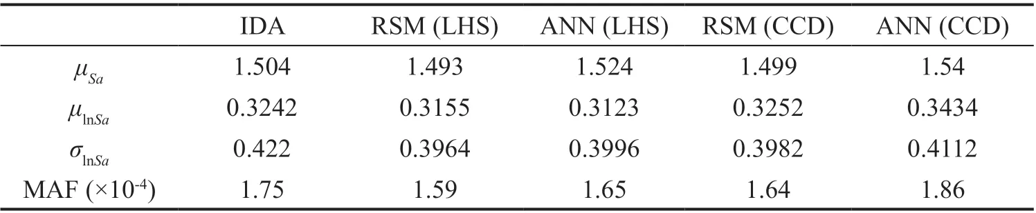
Table 7 Estimated collapse responses when all uncertainties are set to their mean values

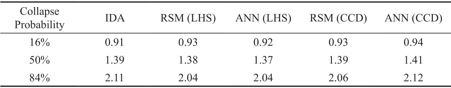
Table 8Sa values correspondingtothecollapseprobabilityatthe levels of 16%, 50% and 84% when alluncertaintiesaresettotheirmean values

Then, 10,000 samples were produced with considering the probability distribution of the uncertainties, and 10,000 more samples were produced without considering the probability distribution of the uncertainties for the 12 epistemic uncertainties. However,since 6,600,000 nonlinear dynamic time-history analyses are required for each of the 10,000 simulations using 44 accelerogram records, and 15 incremental steps for each accelerogram using the Hunt-Fill algorithm, which is very time-consuming, the structural collapse responses are estimated only by the RSM and ANN approaches in a short time. Tables 9 and 10 provide the collapse responses at the levels of 16%, 50%, and 84%. Figures 17 to 20 show the predicted response errors from the IDA values for the 281 simulations.

- At levels of 16%, 50%, and 84%, the maximumμSaerrors for the LHS method and 281 simulations under RSM and ANN were 3.4% and 1.4%, respectively, while for 10,000 simulations under RSM and ANN, they were 2.5% and 1.3%, respectively.

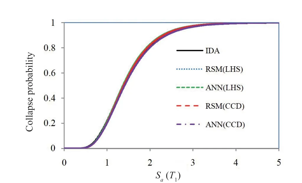
Fig. 15 Estimated collapse fragility curves when all uncertainties are set to their mean values

- The maximum,μSaerrors for the CCD method and 281 simulations under RSM and ANN were 3.3%and 2.2%, respectively, while for 10,000 simulations under RSM and ANN, they were 5.3% and 1.8%,respectively.

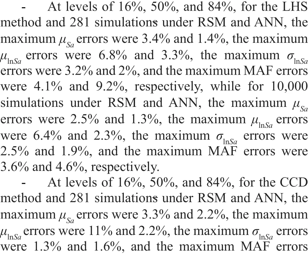
- The maximum,μlnSaerrors for the LHS method and 281 simulations under RSM and ANN were 6.8%and 3.3%, respectively, while for 10,000 simulations under RSM and ANN, they were 6.4% and 2.3%,respectively.

- The maximum,μlnSaerrors for the CCD method and 281 simulations under RSM and ANN were 11% and 2.2%, respectively, while for 10,000 simulations under RSM and ANN, they were 16.7% and 15%, respectively.

- The maximumσlnSaerrors for the LHS method and 281 simulations under RSM and ANN were 3.2%and 2%, respectively, while for 10,000 simulations under RSM and ANN, they were 2.5% and 1.9%, respectively.

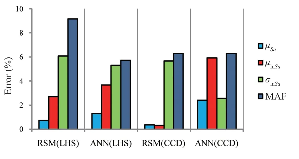
Fig. 16μSa, μlnSa,σlnSa,and MAFerrors when all uncertainties are set totheirmeanvalues

Table 9 Estimation of μSa, μlnSa, σlnSa, and MAF values at the levels of 16%, 50%, and 84% for the LHS method under RSM and ANN

Table 10 Estimation of μSa, μlnSa, σlnSa, and MAF values at the levels of 16%, 50%, and 84% for the CCD method under RSM and ANN

Fig. 17 μSa error at levels of 16%, 50%, and 84%

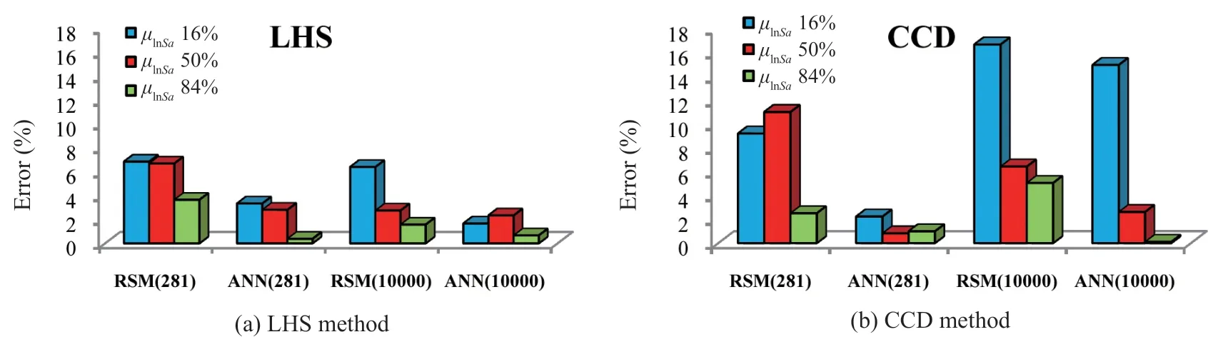
Fig. 18 μlnSa error at levels of 16%, 50%, and 84%

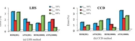
Fig. 19 σlnSa error at levels of 16%, 50%, and 84%

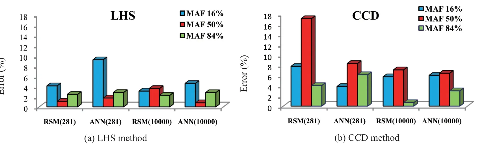
Fig. 20 MAF error at of levels 16%, 50%, and 84%

- The maximumσlnSaerrors for the CCD method and 281 simulations under RSM and ANN were 1.3%and 1.6%, respectively, while for 10,000 simulations under RSM and ANN, they were 1.9% and 3.4%,respectively.

- The maximum MAF errors for the LHS method and 281 simulations under RSM and ANN were 4.1%and 9.2%, respectively, while for 10,000 simulations under RSM and ANN, they were 3.6% and 4.6%,respectively.

- The maximum MAF errors for the CCD method and 281 simulations under RSM and ANN were 17.1%and 8.3%, respectively, while for 10,000 simulations under RSM and ANN, they were 7.1% and 6.4%,respectively.

7 Summary and conclusions

This study was conducted to investigate collapse responses of a concrete moment frame structure by considering model uncertainties. The modeling uncertainties of collapse response evaluation were the parameters of the modified Ibarra-Medina-Krawinkler moment-rotation curve for beams and columns. For the uncertainty analysis, the correlations between the model parameters in a component and two structural components were considered. The Latin hypercube sampling (LHS)method was employed to produce independent random variables with considering the probability distribution of the uncertainties, while the central composite design(CCD) method was used to produce independent random variables without considering the probability distribution of the uncertainties. Next, the Cholesky decomposition was applied to produce dependent random variables for the two simulations. In the first step, 281 random variables were produced for the uncertainties using the LHS method by considering their correlation and IDA was performed with 44 far-fault accelerograms to determine the collapse response of the structure. For the 281 simulations using the 44 selected accelerograms 15 incremental steps for each accelerogram by the Hunt-Fill algorithm, a total of 185,460 nonlinear dynamic timehistory analyses were performed. In the second step, 281 random variables were produced for the uncertainties using the CCD method by considering their correlations.For this purpose, 185,460 new dynamic nonlinear time history analyses were performed. Then, collapse responses were predicted for both simulation modes using RSM and ANN.

To compare the collapse responses of the two simulation modes, the collapse responses were obtained at statistical levels of 0 to 100%. The results revealed that the LHS and CCD correlation coefficients ofμSa,μlnSa,σlnSaand MAF at statistical levels of 0 to 100% are 0.99562, 0.99426, 0.99261, and 0.97955, respectively.Considering that the correlation coefficients were above 0.98 between the collapse responses at statistical levels of 0 to 100% in the two simulation methods, the CCD method can be employed to produce samples for uncertainty analysis and structural collapse response prediction without considering the probability distribution of uncertainties.

Three different tests were performed to compare the prediction methods to the IDA results for both LHS and CCD simulations. The results are as follows:

- When all the uncertainties are set to their mean values, under RSM and ANN, for the LHS method, the maximum errors ofμSa,μlnSaandσlnSawere 6% and the maximum error of MAF was 9%. At the same time, for the CCD method, the maximum errors were 6% forμSa,μlnSaandσlnSaand 6% for MAF.

- TheSaerrors at the collapse probability of 16%,50%, and 84% for the LHS and CCD methods under RSM and ANN were about 3.5%.