Theoretical and experimental studies on critical time delay of multi-DOF real-time hybrid simulation

Lu Liqiao, Wang Jinting, Ding Hao and Zhu Fei

1. State Key Laboratory of Hydroscience and Engineering, Tsinghua University, Beijing 100084, China

2. China Huaneng Group Co., Ltd., Beijing 100031, China

3. Hisense Group Co., Ltd., Qingdao 266520, China

Abstract: This paper aims to investigate the critical stability of a multi-degree-of-freedom (multi-DOF) real-time hybrid simulation (RTHS). First, the critical time-delay analysis models are developed using the continuous- and discrete-time root locus (RL) techniques, respectively. A bilinear transform is introduced into the first-order Padé approximation while conducting the discrete RL analysis. Based on this technique, the time delay can be explicitly used as the gain factor and thus the instability mechanism of the multi-DOF RTHS system can be analyzed. Subsequently, the critical time delays calculated by the continuous- and discrete-time RL techniques, respectively, are compared for a 2-DOF RTHS system. It is shown that assuming the RTHS system to be a continuous-time system will result in overestimating the critical time delay.Finally, theoretically calculated critical delays are demonstrated and validated by numerical simulation and a set of RTHS experiments. Parametric analysis provides a glimpse of the effects of time step, frequency and damping ratio in a performing partitioning scheme. The constructed analysis model proves to be useful for evaluating the critical time delay to predict stability and performance, therefore facilitating successful RTHS.

Keywords: real-time hybrid simulation; root locus; critical time delay; delay-dependent stability

1 Introduction

Real-time hybrid simulation (RTHS) is a promising test method for investigating the dynamic response of complex structures in earthquake engineering. The mechanism of RTHS is used to split the entire structural system into two different parts: the numerical model and the experimental piece. The numerical model is usually the part that can be precisely simulated in computers, while the experimental piece is the one that cannot be simulated, so as to carry out tests instead.The displacement command that is calculated from the numerical model is imposed on the controller so that subsequently the servo-hydraulic system can drive the shaking table or actuator, following a command from the numerical substructure in real time. The measured feedback force at the interface between the numerical and physical substructures is transmitted to the computer in real time for the calculation of the next time step. Such harmonious progress can ensure the stability of RTHS.

During the RTHS test, however, the feedback force from the physical substructure may exhibit a time delay. For a specific control system, a time delay could be caused by control systems, calculation processes or network communications (Magharehet al., 2014).Comparing with the time taken for an actuator-response delay, the calculation/communication delays are quite small. Therefore, the time delay discussed herein refers to the actuator-delay. This inevitable time delay could affect the behavior of the dynamical system and impair the stability and accuracy of RTHS tests. The smallest value of time delay, which leads to instability in the system, is the so-called critical time delay. Accurate prediction of the critical time delay is indispensable to assess the feasibility of performing RTHS tests, set a standard for the servo-hydraulic controllers, and, when necessary, develop a compensation scheme for RTHS.

The stability studies can be divided into two categories based on different system hypotheses:continuous- and discrete-time system analysis.

Many pieces of stability research in single DOF(SDOF) RTHS have been conducted on this problem.For the continuous-time system assumption, Horiuchiet al. (1999) proved that the energy added to the system by time delay is equal to the results taken from equivalent negative damping. To cancel out time delay, Horiuchiet al. proposed a time delay compensation algorithm based on annth-order polynomial function, which has been employed by other researchers (Nakashima and Masaoka, 1999; Darbyet al., 1999; Kobayashi and Tamura, 2000; Blakeboroughet al., 2001; Xuet al.,2016). Magharehet al. (2014) derived a prediction performance index to evaluate the time-delay impact of the actuator for SDOF RTHS and a computational/communication delay regarding the accuracy of RTHS.Such a performance index is adopted along with a stability criterion in the RTHS system (Magharehet al.,2017). Huanget al. (2019) proposed stability criteria through the use of the Lyapunov-Krasovskii theorem and investigated the stability of a linear SDOF system with both a constant and a time-varying delay.

Wallaceet al. (2005) used the delay differential equation (DDE) model of the SDOF system to analyze the influence of an actuator′s time delay in RTHS. A linear mass-spring oscillator system was studied using this approach to define the compensation scheme. Kyrychkoet al. (2006) investigated a pendulum-oscillator system using neutral DDE with a fixed value of time delay.Mercan and Ricles (2007) proposed a method called the pseudodelay technique, which is applicable to pure imaginary poles (Olgac and Sipahi, 2002), to investigate the DDE of elastic SDOF test structures and present the results of amplitude error and time delay in the restoring force. Chenet al. (2017) evaluated the effect of actuator delay on a linear SDOF structure with uncertainty parameters by employing the DDE model. Chiet al.(2010) approximated the exponential time delay using the Padé rational function, and studied the stability of the SDOF system in a continuous time domain. They employed the continuous-time root locus (RL) to investigate the effects of the substructure′s parameters on the system′s stability.

Under the assumption of a discrete-time system, Wuet al.(2005) analyzed the stability and accuracy of the central difference method by using the spectral radius.On the basis of upper bound delay, Wuet al.(2013)investigated the influences of time delay compensation techniques and integration algorithms on the stability of RTHS. Based on the discrete control theory, Chen and Ricles proposed the CR method (Chen and Ricles,2008a) and modeled the actuator delay in a SDOF RTHS system (Chen and Ricles, 2008b).

For the multi-DOF system, the criteria for evaluating the critical time delay should be developed, since studies have shown that the partitioning schemes will affect the stability of the system (Igarashiet al., 2000; Horiuchi and Konno, 2001). Mercan and Ricles (2008) researched the stability boundary of 2-DOF and 3-DOF RTHS systems in a continuous-time domain with multi-source delays. Huanget al. (2020) extended the stability criteria(Huanget al., 2019) to a linear multi-DOF structure with multiple actuator delays. Zhuet al. (2015, 2016)selected the mass ratio between physical and numerical substructure as the indicator for depicting stability performance using discrete-time RL. Though many pieces of research have been done in the field of stability of RTHS, critical time delay has not been investigated using the discrete-time technique for the multi-DOF RTHS. The difference between the continuous- and discrete-time assumptions when determining the critical time delay has also rarely been investigated.

In the present study, a critical time-delay analysis model for multi-DOF RTHS based on both continuousand discrete-time RL is developed, and is fully implemented as a criterion to examine the stability of a linear system under time delay. In the continuoustime RL analysis, the first-order Padé approximation is used as the s transform of time delay. In the discretetime RL analysis, we introduce the bilinear transform into the first-order Padé approximation to obtain the z transform of time delay. This makes it possible to select the time delay as the gain factor in the continuous- and discrete-time RL equation. The critical time delays for the multi-DOF system with a pure time delay are investigated based on the critical time-delay analysis model, and the stability principle is studied and verified by the numerical simulation and RTHS experiments,respectively. Moreover, parametric analysis is performed to provide a comprehensive study on critical time delay.The successful performance of a series of validation experiments is encouraging and the multiple-trial experience accompanied by the critical analysis model may help facilitate assessing the unstable oscillation or performance degradation of RTHS.

2 Critical time-delay analysis model using the RL technique

2.1 Introduction to continuous-and discrete-time RL rules

In automatic control engineering, RL analysis is a tool for assessing closed-loop system performance. The RL technique includes two methods: continuous- and discrete-time RL. The continuous-time RL is on an s-plane through the Laplace transform of the results in time domain, while the discrete-time RL is a z-transform on the z-plane. The s- and z-transforms can be converted to each other.

As can be seen in Fig. 1, the RTHS system also belongs to the closed-loop system, in which the dynamic characteristics depend on theGclin Eq. (1).

The closed-loop transfer functionGclis defined as,

whereXiandFiare the s- or z-transform ofX(t) andF(t);GHis the open-loop transfer function; and 1 +GH= 0 is the characteristic equation (also known as root locus equation). As a property of the system itself, transfer functionGclis independent of the form and size of the input load.

The s- and z-transform have the advantage of using this transformation to convert a signal from the timedomain to the s- or z-domain, which in turn convert the differential equation or difference equation into an algebraic equation to describe the characteristics of the system, thereby simplifying the calculation.

When the initial condition is zero, suppose that the sampling period of the discrete-time seriesx(t) is Δt, the corresponding s- and z-transform ofx(t) are defined as,respectively,

whereKclis the gain factor of the system and varies from 0 to +∞,siandpjis the zero and pole of the open-loop transfer function for the continuous-time RL;ziandqjis the zero and pole of the open-loop transfer function for the discrete-time RL;m0andn0are positive integers.

Fig. 1 The closed-loop transfer function system

For a linear time-invariant closed-loop system,its stability is judged by the poles and zeros of the characteristic equation. Figure 3 shows the so-called pole-zero map of the continuous- and discrete-time RL in the s- and z-planes. A circle (°) and a cross (×) can be used to mark the corresponding zero location and pole location, which provide an intuitive insight into the dynamic response of the system. The location of these poles changes as gain factorKclincreases from 0 to +∞.A locus of these poles plotted as a function ofKclis known as a RL. Each RL begins at the open-loop pole and ends at the open-loop zero (i.e., mode 1 in Fig. 3).If the number of poles of the system exceed zero, then some of the loci end at infinity (i.e., mode 2 in Fig. 3).The left-hand side of the s-plane (inside the unit circle in the z-plane) is a stable region, while the right-hand side of the s-plane (outside the unit circle in the z-plane)is an unstable region. If the RL across the imaginary axis in the s-plane (the unit circle in the z-plane), the intersection point is named as a critical stability point.The critical stability point is regarded as unstable in classical control theory. The critical stability point stands for the critical time delayτcrwhen the time delay is chosen as gain factorKcl. In this paper the critical time delayτcris adopted to represent the lower limit of a time delay that causes instability in the system.

2.2 Critical time-delay analysis model

Based on the introduction of the RL technique in Section 2.1, the critical time-delay analysis model of the multi-DOF is proposed herein.

The equations of motion in the system may be represented as,

Then the equations of motion for anM-storey shear frame withM-DOFs can be rewritten as

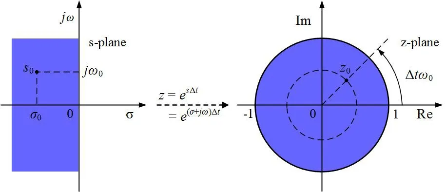
Fig. 2 The mapping relation between the s-plane and the z-plane

Fig. 3 Schematic diagram of the continuous- and discrete-time RL in the s-and z-planes

The Gui-λmethod (Guiet al., 2014) is adopted herein as the integration method,

Whenn≤ 6, the coefficient in Eq. (15) results are summarized in Table 1.

The accuracy of the Padé approximation is related to the parameters, including number of order, time delay and frequency. MATLAB offers the Pade function to return phase responses ofNth-order Padé approximation and compare it with the exact response, evaluating the phase error when the number of order and time delay are specified (Mathworks, 2019a). Based on the concerned time delay herein, an illustration of the theoretical analysis of the Padé approximation is shown in Fig. 4.It can be seen that the phase error will increase with an increase in the frequency and time delay. For the servo-hydraulic system with which we have used in our investigation, the time delay is 0-20 ms, and the frequency span is 0-20 Hz. Therefore, the first-order Padé approximation is feasible for retaining accuracy in this case.

when a time delay exists, we introduce the time delay formula (Eq. (16)) into the characteristic Eq. (13). In the form of Eq. (4), the RL equation can be rewritten as follows:

The coefficients of the RL equation Eq. (17) are summarized in Table 2.

2.2.2 Discrete-time RL technique

To study the dynamic response of the system in adiscrete-time manner, the Gui-λmethod is selected herein as the numerical integration method. The z-transform of Eq. (9) is,

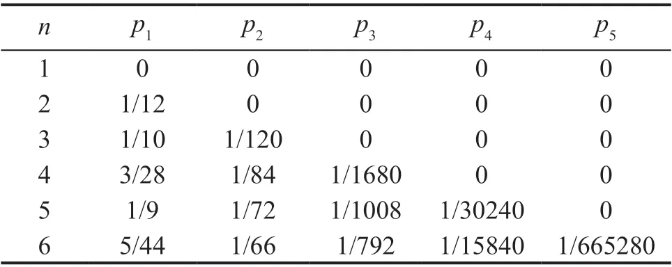
Table 1 Coefficients of the Padé function (n ≤6)

Table 2 Coefficients of the continuous-time RL equation

whereh(z) is the z-transform of the time delay.

The corresponding closed-loop transfer function is

h(z) in Eq. (23) is a transcendental equation.Therefore, instead of using Eq. (23), the bilinear transform is incorporated herein into the first-order Padé approximation to obtain the rational expression ofh(z)and deduce the characteristic equation with regard to time delay.

Fig. 4 Phase error evaluation for the first-order Padé approximation

The bilinear transform (also known as Tustin′s method) yields the best match in frequency domain between the z- and s-transforms (Mathworks, 2019b),and the formula is as follows:

The bilinear transform will lead to a warping in the frequency domain. The allowable area for a good bilinear transform approximation is inversely proportional to the time step (Houpis and Sheldon, 2013); thus, the selected time step will affect the obtained critical time delay.Besides, MATLAB offers the functionc2dto discretize a continuous-time model (Mathworks, 2019b). The system response betweenh(s) andh(z) is compared using a constant time delayτ= 22/2048 s under three time-steps as shown in Fig. 5. The curves ofh(s) andh(z) coincide well within the concerned frequency span 0-100 rad/s. Therefore, Eq. (25) is able to represent the time delay in the z domain at a high level of accuracy for the discussed frequency range.

When a time delay exists, the time delay formula(Eq. (25)) is introduced into the characteristic equation(Eq. (22)). According to the form of Eq. (5), the RL equation is written as follows:

The coefficients of the RL equation Eq. (26) are provided in Table 3.

Based on the critical time-delay analysis model (17)and (26), the critical time delay of multi-DOF systems could be analyzed through use of the RL technique. The instance analysis will be studied using the proposed critical time-delay analysis model in the following sections. Meanwhile, the corresponding numerical and experimental verification will also be presented thereafter to prove the feasibility of the proposed model.

3 Stability analysis of a 2-DOF system

Since the 2-DOF structure is the simplest type of the multi-DOF systems, a 2-DOF frame model is adopted herein to understand and compare the critical time delay of multi-DOF RTHS systems through the use of the continuous- and discrete-time RL technique, and its parameters are summarized in Table 4.

The continuous- and discrete-time RLs are discussed,respectively, to compare the differences between these two methods.

Case A: Continuous-time RL.

Figure 6 shows the analytical results of the continuoustime RL. It can be seen that the emulated system has two modes. For each mode, the circular frequency at the open-loop pole is equal to that of the emulated system,which means that these two modes correspond to the system′s inherent modes. Therefore, such modes are called Inherent Mode 1 and 2, respectively. In addition to the inherent modes, there is also an added mode caused by the time delay (Chiet al., 2010). Inherent Mode 1 always lies in the left half of the s-plane as the time delay increases. Whenτ= 6.28 ms, Inherent Mode 2 crosses the imaginary axis, resulting in the instability of the system. This suggests that an increase in the time delay will lead to system instability. The critical time delay of the emulated system isτcr= 6.28 ms, and its critical circular frequency isωcr= 50.86 rad/s.

Fig. 5 Phase error evaluation for the bilinear transform(τ = 22/2048 s)

As for the discrete-time RL, the following three cases are adopted to study the impact of the time step on the critical time delay.

Case B-1: Discrete-time RL. Time step Δt= 2/2048 s (0.001 s)Case B-2: Discrete-time RL. Time step Δt= 10/2048 s(0.005 s)

Case B-3: Discrete-time RL. Time step Δt= 20/2048 s(0.01 s)

The 2-DOF frame model in Table 4 is investigated.The system RL diagram can be viewed in Figs. 7-9.

Figure 7 shows the analysis results of Case B-1. In the z-plane, Inherent Mode 1 always remains inside the unit circle as the time delay increases, while Inherent Mode 2 crosses the unit circle at pointτ= 6.24 ms, resulting in the instability of the system. The critical time delay and the critical circular frequency of the emulated system areτcr= 6.24 ms,ωcr= 50.85 rad/s, respectively.

The system performance for Case B-2 is shown in Fig. 8. The RL has similar path with Case B-1. Inherent Mode 2 crosses the unit circle at pointτ= 6.08 ms,resulting in the instability of the system. The critical time delay and the critical circular frequency of the emulated system areτcr= 6.08 ms,ωcr= 50.60 rad/s.

The stability analysis of Case B-3 is plotted in Fig. 9.Inherent Mode 2 crosses the unit circle at pointτ= 5.72 ms,which causes instability in the system. The critical time delay and the critical circular frequency of the emulated system areτcr= 5.72 ms,ωcr= 49.86 rad/s.

It can be seen from Figs. 7-9: (1) The critical time delay will decrease as the time step increases. This means that the large time step will increase the instability of the hybrid simulation system. (2) The RL will be farther from the real axis as time step grows.

The critical time delay RL plots in Figs. 6-9 reveal that the time delay impact on Inherent Mode 2 is the main cause of the system instability. Furthermore,the mechanism of system instability is analyzed by investigating the equivalent damping ratioζeq. According to the poles′ location on the z-plane, the equivalent damping ratioζeqis computed based on the formula as follows (Chen and Ricles, 2008b):

NumeratorDenominator n34M + 2ΔtC + Δt2Kd3(4M + 2ΔtC + Δt2K)Δt n2-12M - 8ΔtC2 - 2ΔtC+Δt2 K1 - 7Δt2K2d2-4M + 2ΔtC + 3Δt2K n112M - 2ΔtC1 + 14ΔtC2 - Δt2K1 + 7Δt2K2d1-4M - 2ΔtC + 3Δt2K n0-4M + 2ΔtC1 - 6ΔtC2 - Δt2Kd0(4M - 2ΔtC + Δt2K) Δt

Table 4 Parameters of the 2-DOF model

Fig. 6 The 2-DOF system′s critical time delay of the continuous-time RL plot

whereσandεare the pole′s real and imaginary coordinates in RL.

The results of the equivalent damping ratioζeqare plotted with respect to time delayτin Fig. 10 for Case A,and Case B-1 to B-3.

From Fig. 10, it can be seen that in Case B-1 to B-3,the equivalent damping ratioζeqwill increase with the increase of time delayτin Inherent Mode 1. For Inherent Mode 1, the all along positive value of the equivalent damping ratioζeqwill not hamper the stability of the entire system. In addition, the equivalent damping ratioζeqwill decrease with the increase of time delayτin Inherent Mode 2. The equivalent damping ratioζeqwill be zero at the critical time delayτcrpoint, so that the system will be unstable. Therefore, the reason for the instability of the 2-DOF system is that the equivalent damping ratio will be reduced to zero, caused by a time delay in Inherent Mode 2.

According to the control theory, the increase of the time step will leave more adverse effects on stability.Compared with Case A and three cases in Case B, it should be concluded that: (1) the equivalent damping ratio of continuous- and discrete-time RL demonstrates similar variation trends; (2) assume the RTHS system as a continuous-time system will overestimate the critical time delay; and (3) in the discrete-time RL, the increase of time step will decrease the critical time delay of the hybrid simulation system.

Fig. 7 The 2-DOF system′s critical time delay of the discrete-time RL plot (Δt = 2/2048 s)

Fig. 8 The 2-DOF system′s critical time delay of the discrete-time RL plot (Δt = 10/2048 s)

Fig. 9 The 2-DOF system′s critical time delay of the discrete-time RL plot (Δt = 20/2048 s)

4 Numerical verifications of the critical timedelay analysis model

The numerical model is adopted to verify the critical time delay results calculated by the RL technique in this section. The parameters of the model shown in Table 4 are used. As the flow chart shows in Fig. 11, the entire system is numerically simulated by using MATLAB/Simulink software. The unit delay block can implement the time delay in the Simulink simulation.

Two sets of simulations are performed with the dynamic base excitation, including a sinusoidal sweep wave and El Centro ground motion. The Gui-λmethod withλ= 4 is chosen to analyze the structural dynamic response. The calculation time step is kept at Δt= 10/2048 s.The first two natural frequencies of the model are 3.1 Hz and 8.1 Hz, separately. The damping ratio isζ= 4.4%,and Rayleigh damping is adopted. The system’s time delay is assumed to beτ= 10/2048 s, 20/2048 s, 40/2048 s,respectively.

4.1 Sinusoidal sweep excitation analysis

A swept-frequency sinusoidal wave with an amplitude of 0.15 g varying from 1 Hz to 10 Hz is used as the base excitation. The sweep frequency is 0.45 Hz/s,as shown in Fig. 12.

Figure 13 presents the displacement response and Fourier spectrum of the system with a delay of 10/2048 s. The dynamic responses of DOF2 for the 2-DOF structure under sinusoidal sweep excitation without time delay are taken as the Target results. The responses of the system under time delay have obvious differences with the target when no delay occurs. As shown from the displacement time history in Fig. 13(a), the divergence of the second-order dynamic response results in the instability of system, which demonstrates that the decline of the equivalent damping ratio for the Inherent Mode 2 under time delay may render the RTHS test to be unstable, as described in Section 3.

Figures 14 and 15 show the displacement time history of the system when the time delay isτ= 20/2048 s and 40/2048 s, respectively. It can be observed that the responses of the system are both divergent, and increasing the time delay will result in more rapid instability.

Consistent with the critical time delay of the emulated systemτcr= 6.08 ms, the 2-DOF structure remains stable with a delayτ= 10/2048 s (<τcr), and obviously turns unstable with a larger delayτ= 20/2048 s (>τcr). Therefore,the sinusoidal sweep excitation test proves the feasibility of the critical time-delay analysis model.

4.2 Earthquake excitation analysis

The El Centro ground motion with an amplitude of 0.5 g is used as the external excitation in this simulation test. The time history and Fourier spectrum of the seismic wave is shown in Fig. 16.

The displacement time history and Fourier spectrum of the system for a time delayτ= 10/2048 s are illustrated in Fig. 17. The Target results (drawn with a solid line)represent the dynamic response of DOF2 for the 2-DOF structure without a time delay. The dynamic responses both are divergent in Figs. 18 and 19 when the time delay isτ= 20/2048 s and 40/2048 s.

Based on the results of the numerical test using a sinusoidal sweep wave and El Centro ground motion excitation, as described above, the dynamic responses of the 2-DOF system are convergent, with a time delayτ= 10/2048 (<τcr), and divergent whenτ= 20/2048(>τcr). These conclusions conform with the stability criterion from the critical time-delay analysis model found in Section 3.

5 Parametric analysis of the critical time delay

Fig. 10 Variation of the 2-DOF system′s equivalent damping ratio with the time delay τ

Fig. 11 Flow chart of numerical verification

Fig. 12 Swept-frequency sinusoidal wave

Fig. 13 Dynamic response of DOF2 for a 2-DOF structure under sinusoidal sweep excitation (τ = 10/2048)

The effects of structural parameters (i.e., frequency,damping ratio) and time step on the critical time delay of the 2-DOF system when performing the partition configuration are investigated herein. It is assumed that the damping ratio of the physical substructure is the same as the numerical one, i.e.,ζP=ζN=ζ. The frequency ratio of the physical and numerical substructure isA=ωP/ωN,i.e.,ωP=Aωn,ωN=ωn, where subscriptPindicates the physical substructure, subscriptNrefers to the numerical substructure, andωnranges from 0 to 314 rad/s.

5.1 Time step analysis

The analysis procedure in this section will show the effects of time step on the critical time delay of the system,starting with the assumption of the structural properties as follows: the damping ratioζ= 0.044; the frequency ratio is set asA= 0.5, 1, 2 and 4. The time step is chosen as Δt= 0.001 s, 0.005 s and 0.01 s, respectively. Figure 20 shows the trend of the critical time delayτcrwhen the circular frequencyωnrises from 0 to 314 rad/s. Both the continuous- and discrete-time results are shown in this figure to demonstrate the effects of the two assumptions made on the critical time delayτcr.

As can also be seen in Fig. 20, the critical time delay of the continuous-time RL is almost the same with the discrete-time RL, with Δt= 0.001 s. This means that when time step Δtis sufficiently small, the system can be considered as a continuous-time system. This also verifies the accuracy of the discrete-time RL. The critical time delay will decrease with the increase of the time step in discrete-time RL. This shows that the discretization of the numerical methods will reduce RTHS system stability. The continuous-time RL results are not safe enough for the reference of RTHS experiments. When the time step Δtin the numerical methods is large, the discrete-time RL should be chosen to predict the stability of the RTHS system.

The critical time delay will decrease with an increase in the valueA, which means overall low frequency is a benefit for the stability of the entire structure.

5.2 Damping ratio analysis

This section will illustrate how the damping ratio of the structure impacts the critical time delay of the linear 2-DOF system. The following parameters are employed herein: the time step of the discrete-time RL is Δt= 0.005 s,the damping ratioζ= 0.01, 0.044, 0.1, and the frequency ratioA= 0.5, 1, 2 and 4. As can be seen from Fig. 21, the critical time delay will decrease with an increase of the circular frequencyωn, which varies from 0 to 314 rad/s.

Fig. 14 Dynamic response of DOF2 for a 2-DOF structure under sinusoidal sweep excitation (τ = 20/2048)

Fig. 15 Dynamic response of DOF2 for a 2-DOF structure under sinusoidal sweep excitation (τ = 40/2048)

The critical time delay will obviously increase with an increase in the damping ratioζ, which means that damping ratioζcan significantly improve the stability of the system. As can be seen in Fig. 21, the critical time delay will decrease with an increase in the frequency ratioA, which verifies that a physical substructure with low frequency is good for the stability of the entire structure. The discrete-time RL will reduce the critical time delay compared with the continuous-time RL.

The critical time-delay analysis model is useful,considering that the time delay is key to the stability of the RTHS experiment. Based on the proposed analysis model, the stability of the RTHS can be judged by the relationship between the time delay in RTHS tests and the critical time delay calculated by this particular technique,thus providing guidance for partitioning choices and implementation of the compensation method.

6 Experimental verification

Fig. 16 Time history and Fourier Spectrum of El Centro ground motion

Fig. 17 Dynamic response of DOF2 for a 2-DOF structure under El Centro ground motion (τ = 10/2048)

Fig. 18 Dynamic response of DOF2 for a 2-DOF structure under El Centro ground motion (τ = 20/2048)

Fig. 20 The critical time delay of the 2-DOF system with ζ = 0.044: (a) ωP = 0.5ωN; (b) ωP = ωN; (c) ωP = 2ωN; (d) ωP = 4ωN

Fig. 19 Dynamic response of DOF2 for a 2-DOF structure under El Centro ground motion (τ = 40/2048)

Fig. 21 The critical time delay of the 2-DOF system with Δt = 0.005 s: (a) ωP = 0.5ωN; (b) ωP = ωN; (c) ωP = 2ωN; (d) ωP = 4ωN

Fig. 22 Outline of the D-RTHS system

The RTHS system with dual target computers(D-RTHS) is adopted to verify the feasibility of the proposed critical time-delay analysis model. As shown in Fig. 22, the D-RTHS system includes three parts: the distributed real-time calculation system, the shaking table loading system, and the data acquisition and transmission system. The distributed real-time calculation system divides the calculating task into the response analysis task(RAT) and the signal generation task (SGT) (Nakashima and Masaoka, 1999). The numerical substructure is solved on Target Computer 1 with a main time step(RAT), and the displacement signal is implemented with a sub time step on the Target Computer 2 (SGT). The sampling frequency of the shaking table loading system is 2048 Hz. In the data acquisition and transmission system, the data is transmitted in real-time through three installed SCRAMNet cards. Details of the system can be referred to in Zhuet al. (2014).

In this experiment, both the main time step Δt, and the sub time step δtare set as 1/2048 s to avoid any additional time delays. The Gui-λmethod (λ= 4) (Guiet al., 2014) is chosen as the integration method.

6.1 RTHS experimental setup

As shown in Fig. 23, a RTHS system involving a two-story shear frame is investigated herein. The upper story frame acts as the physical substructure, which has been investigated in previous studies (Luet al., 2018),and the lower story is numerically simulated. The mass,fundamental frequency and damping ratio of the physical substructure aremP= 5.28 kg,fP= 5.8 Hz, andζP= 4.4%,respectively. The frequency and the damping ratio of the numerical substructure is the same as the physical one,i.e.,fN=fP,ζN=ζP. The mass of the numerical substructuremNis chosen to arrive at the desired mass ratio.

The sinusoidal wave load is adopted as the external excitation to the system. An amplitude of 0.025 g for the excitation is selected to ensure that the entire structure demonstrates linear behavior.

6.2 Experimental results

To precisely verify the critical time delay of the RTHS system, it is necessary to specify an appropriate time delay, which would be near the critical stability state.Considering that the inherent time delay from the servohydraulic system is around 22/2048 s (≈11 ms) (Zhuet al., 2017), ten cases, defined as Cases C-1 to C-10, with a critical time delay increment by 1 ms, are created by adjusting the mass of the numerical substructure. The corresponding parameters of these ten cases are listed in Table 5. The theoretical critical time delay is calculated by the proposed critical time-delay analysis model within the discrete-time domain, with a time step of 1/2048 s.Even though the critical time delay is examined herein by adjusting the mass of the numerical substructure, it is feasible to apply other structure parameters (damping,frequency, etc.) using the analysis model as a guideline to demonstrate stability and performance.

Ten validation experiments conforming to Cases C-1 to C-10 are implemented to demonstrate the stability performance of the RTHS system. The results show that the dynamic responses of the ten cases can be divided into three types: (a) stable stage and desirable results are achieved (C-1, C-2); (b) test does not fail but the accuracy of the experimental results declines (C-3, C-4);(c) test fails and the instabilities increase with a decrease in critical time delay (C-5 to C-10).

Among these ten cases, Cases C-1, 4, 6 and 10 are chosen to depict the dynamic responses of RTHS system change from stable, to precision declines, to fail gradually/immediately. The experiment results at the interface between the numerical and physical substructure are plotted in Figs. 24 to 27. Displacement time history and the Fourier Spectrum are given to demonstrate the stable tests, while both the displacement and acceleration responses are plotted for an analysis of the unstable ones.The two-story emulated system without a time delay is calculated in Simulink for comparison.

From the displacement time history and the spectrum analysis for Case C-1 shown in Fig. 24, it can be observed that the dynamic responses are steady.The RTHS experimental results coincide well with the numerical simulation.

It can be seen in Fig. 25 that although the test did not fail in Case C-4, both the displacement and acceleration time history are undesirable. From the Fourier Spectrum of displacement and acceleration shown in Fig. 25(b)and 25(d), the experimental unstable frequency is 39.28 rad/s, which agrees well with the theoretical valueωcr= 44.01 rad/s in Table 5.

The test failed in Case C-6 since the critical time delayτcris near the inherent time delay of the hydraulic system. Displacement and the acceleration time history are gradually divergent and eventually lead to an interruption in the experiment. The unstable frequency from the displacement and the acceleration Fourier Spectrum is 39.67 rad/s, which is close to the computed critical circular frequencyωcr= 45.60 rad/s in Table 5.

Fig. 23 Schematic diagram of the frame system setup for RTHS: (a) split of substructures, and (b) photograph of the physical substructure

Table 5 Parameters of the two-story shear frame RTHS system for Cases C-1 to C-10

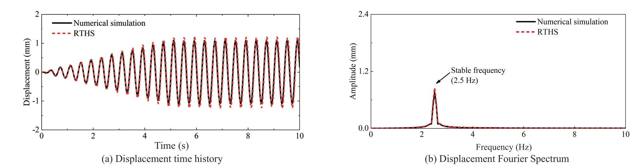
Fig. 24 Dynamic responses at the bottom of the steel frame in Case C-1

Fig. 25 Dynamic responses at the bottom of the steel frame in Case C-4

Figure 27 presents the dynamic responses for Case C-10. Both the displacement and acceleration response are divergent immediately after the test starts due to a small critical time delayτcr= 7 ms. The correspondingly unstable frequency is not computed since the time histories are short in this instantaneous interruption.

The differences in unstable frequency and displacement response between RTHS tests and the numerical simulation are summarized in Table 6.For stable test C-1, the error in the peak value of the displacement response is 13.50%. The unstable frequency obtained from the analysis model and the experiment is 44.01 rad/s and 39.28 rad/s for test C-4. For the failed test C-6, the unstable frequency is 45.60 rad/s from the critical time-delay analysis model and 39.67 rad/s from experiments. Therefore, the unstable frequency computed from the critical time-delay analysis model agree well with those from the RTHS tests.

From the ten experiments above we can see that the critical time-delay analysis model can provide a match criterion for the stability of real RTHS tests. To ensure that a RTHS test is performed in the stable and accurate stage (a), a minimum tolerance of 4-5 ms should be considered higher than the result of the critical time delay model. It should be noted that this proposed tolerance is from multiple-trial experience and the value may change according to the design of different RTHS systems.

The factors destabilizing the RTHS experiments are much more complicated; therefore, this paper simplifies the factors and the critical time-delay analysis model to provide a practical method for referencing the stability criterion for a linear RTHS system. The critical timedelay characteristics of RTHS configuration that are involved with nonlinear substructures will be studied in future research.

Fig. 27 Dynamic responses at the bottom of the steel frame in Case C-10

7 Conclusions

In this study, the critical time delay in multi-DOF RTHS systems is compared through the use of the continuous- and discrete-time analysis model. The following conclusions are drawn:

(1) The analysis model presents a reliable approach for analyzing critical time delay during a linear RTHS test. In the critical time-delay analysis model, the firstorder Padé approximation is adopted to enable the continuous-time characteristic equation with regard to time delay, while the bilinear transform is introduced into the first-order Padé approximation to deduce the discrete-time characteristic equation while conducting RL analysis. The critical time-delay analysis model is suitable for low frequency (0-20 Hz) and small delay(0-20 ms) cases due to the use of the Padé approximation and bilinear transform.

(2) Approximating the RTHS system as a continuoustime system will overestimate the critical time delay. The equivalent damping ratio of continuous- and discretetime RL demonstrates similar variation trends.

(3) The critical time-delay analysis model using the RL technique provides a preliminary guideline for the stability and performance of the RTHS system, which is demonstrated and validated both by numerical simulation and a series of experiments. Based on the results of the critical time-delay analysis model, experiments showthat additional tolerance is necessary for a reliable and accurate RTHS of a linear system. Regardless, the analysis model may be used to examine the partitioning choices when designing RTHS tests.

Table 6 Comparison between numeration and experiment in Cases 1, 4, 6, 10

Acknowledgement

This research is financially supported by the National Natural Science Foundation of China (Nos. 51725901 and 51639006). The authors express their sincerest gratitude for the support.