An Efficient Algorithm for Low Rank Matrix Restoration Problem with Unknown Noise Level

WANG Duo SHANG You-linLV Jin-man

(1.School of Mathematics and Statistics,Henan University of Science and Technology,Luoyang 471023,China;2.LMIB of the Ministry of Education,School of Mathematical Sciences,Beihang University,Beijing 100191,China;3.State Key Laboratory of Rail Traffic Control and Safety,Beijing Jiaotong University,Beijing 100044,China;4.School of Mathematics and Statistics,Wuhan University,Wuhan 430072,China)

Abstract:Recovering an unknown high dimensional low rank matrix from a small set of entries is widely spread in the fields of machine learning,system identification and image restoration,etc.In many practical applications,the few observations are always corrupted by noise and the noise level is also unknown.A novel model with nuclear norm and square root type estimator has been proposed,which does not rely on the knowledge or on an estimation of the standard deviation of the noise.In this paper,we firstly reformulate the problem to an equivalent variable separated form by introducing an auxiliary variable.Then we propose an efficient alternating direction method of multipliers(ADMM) for solving it.Both of resulting subproblems admit an explicit solution,which makes our algorithm have a cheap computing.Finally,the numerical results show the benefits of the model and the efficiency of the proposed method.

Keywords:Matrix restoration;Alternating direction method of multipliers;Square root least squares;Matrix completion

§1.Introduction

The problem of recovering a high dimensional matrix from noisy observations with unknown variance of the noise arises in many applications such as system identification,machine learning and image processing,etc[2,20,22].For the high dimensional setting,the unknown matrix always has the exactly or near low rank property.Thus the high dimensional low rank matrix estimation from noisy observations has been attracting much attention,such as its two particular settings of the matrix completion(MC) and the multivariate linear regression [17].In this paper,we focus on solving the problem of low rank matrix completion and its general form with unknown noise level,which are widely applied in collaborative filtering and machine learning [4,18,19,23].The mathematical model of MC with noiseless can be formulated as

whereMis the real unknown matrix with some available sampled entries and Ω is a given set of index pairs (i,j).Its general form is the following matrix rank minimization problem

whereA:Rm×n →Rpis a linear map andb∈Rpis a given measurement vector.The rank minimization problem of (1.1) and (1.2) are regarded as NP-hard problems because of the combinatorial properties of rank function [21].For solving these problems more efficiently,a popular method is to use the nuclear norm of the matrix instead of its rank,which is the best convex relaxation of the rank function over the unit ball of matrices with norm less than one[21].Then the problem (1.2) can be transformed into

The nuclear norm ofXis defined as the sum of its singular values,i.e.,,where theσ1≥σ2≥···≥σr>0 are therpositive singular values of the matrixX.In practice,if the measurementbcontains a small amount of noise,the problem (1.3) can be relaxed to the following inequality constrained nuclear norm minimization problem

or its equivalent nuclear norm regularized least square problem

whereδ ≥0 reflects the noise level andµ>0 is a regularization parameter.

The above nuclear norm minimization problems have been widely studied in recent years.Given the problems are convex,they have been solved by many efficient algorithms such as SeDuMi [27] and SDPT3 [31],singular value thresholding(SVT) algorithm [3],fixed point continuation with approximate SVD(FPCA) method [21],accelerated proximal gradient(APG)[30] method,ADMM type algorithms [6,14,16,26,33],etc.

It is clear to see that most of above proposed noisy models have considered using the squaredl2norm to fit the data fidelity term,which can deal with the noiseless and Gaussian noisy problem effectively.Moreover,the recovery of theXrelies on knowing the standard deviation of the noise for the noisy case.However,in practical applications,the noise level is often unknown or is non-trivial to estimate when the problem scale is large.Therefore,there is a certain gap between the theory and the practice.Previously many researchers have studied the multivariate linear regression with unknown noise variance [12,32].The scaled Lasso [24] and the penalized Gaussian log-likelihood [25] have been presented for dealing with the unknown noise level in high dimensional sparse regression.Fonseca and Mark [9] firstly proposed a square-root Lasso method for estimating high-dimensional sparse linear regression models.Bellec et al [1] and Derumigny [5] showed that the square root Lasso can achieve the minimax optimal rate of convergence under some suitable conditions,even though the noise level is unknown.And the square root Lasso model is essentially equivalent to the scaled Lasso proposed by Sun and Zhang [28].Recently,Tang et al [29] considered the high-dimensional nonconvex square root loss regression problems and introduced a proximal majorization-minimization algorithm for solving these problems.Given the above research,we know that the choice of the regularized parameter is usually related to the level of the noise,and the advantage of choosing the square root norm is that choosing the regularized parameter does not rely on the knowledge or on an estimation of the standard deviation of the noise.Previously,multivariate linear regression(matrix regression)with unknown noise variance was considered in[2,11],which studied the rank penalized estimators.They need a assumption on the dimensions of the problem and the rank of the unknown matrix,respectively.Thus a new method by using the Frobenius norm instead of the squared Frobenius norm is proposed in the literature [17],which needs weaker conditions than the conditions obtained in [2,11].They considered the matrix completion problem and the matrix regression problem,and reformulate the low rank matrix completion problem as

where the observationb∈Rpmay contain some noise andµ>0 is a given regularized parameter,||·||2is the Euclidean norm of vector.When theAis a linear operator to pick up the entries in index pairs Ω from a matrix,the problem(1.7)reduces to the MC problem.It is clear to see that the problem (1.7) isn’t easy to solve due to the nonsmooth terms in the objective function.Thus we firstly add a new variable and transfer the model (1.7) to its augmented Lagrangian form.Then we split the task of minimizing the corresponding augmented Lagrangian function into two subproblems.The resultingy−subproblem has closed-form solution,and the closed-form solution of theX−subproblem can also be easily derived by linearizing the quadratic term.So the proposed algorithm is easily performed and makes each subproblem easier to be solved.

The main purpose of this paper is to introduce an ADMM for solving the model (1.7),which can deal with the high dimensional matrix restoration problem with unknown noise level.Moreover,the convergence results are given.The advantage of the model and the efficiency of the proposed algorithm are presented and demonstrated by some numerical experiments.

The rest of this paper is organized as follows.In Section 2,we construct the ADMM for problem (1.7),and give the convergence of the proposed algorithm.The numerical results are reported in Section 3.Finally,we conclude the paper in Section 4.

§2.Algorithm

In this section,we will briefly review some typical ADMM firstly,and then show how to employ ADMM to solve the problem (1.7).Finally,we give the convergence result of the proposed method.

2.1.Review of ADMM

LetX,Y,Zbe finite dimensional real Euclidian spaces.Consider the following convex optimization problem with two block separable structure

wheref:Y →(−∞,+∞] andg:Z →(−∞,+∞] are closed proper convex functions,A:X →YandB:X →Zare given linear maps,with adjointsA∗andB∗respectively,andc∈Xis given data.The augmented Lagrangian function associated with (2.1) is

wherex∈Xis a multiplier,β>0 is a given penalty parameter.Starting from (x0,y0,z0)∈X×(dom f)×(dom g),the general iterative scheme of ADMM for solving (2.1) can be expressed as

where theξis a step-length,which is chosen in the intervalIt is well known that the iterative scheme(2.3)is exactly the classical ADMM introduced by Glowinski&Marroco[13]and Gabay &Mericire [10] whenTf=0 andTg=0.WhenTfandTgare positive definite andξ=1,it becomes the proximal ADMM of Eckstein [7].When bothTfandTgare self-adjoint positive semi-definite linear operators,it turns into the semi-proximal ADMM of Fazel et al [8].

2.2.Algorithm

In this subsection,we employ the ADMM for solving the problem (1.7).Given an auxiliary variabley=A(X)−b,the problem (1.7) can be transformed equivalently into

The corresponding augmented Lagrangian function of (2.4) is

wherez ∈Rpis the Lagrangian multiplier andβ>0 is a penalty parameter.Given (Xk,yk,zk),we obtain (Xk+1,yk+1) by alternatively minimizing (2.5),i.e.,

Firstly,for the given{(Xk,yk)},we can obtainXk+1by minimizing (2.5) with respect toXas follow:

However,its analytic solution is not clear because of the linear mappingA.Letgk=A∗(A(Xk)−) be the gradient ofatXk.Instead of solving (2.7),the Xsubproblem can be solved by an approximated model,i.e.,

To get the exact solution of (2.8),letY=Xk −τgk,then the solution ofX-subproblem can be reformulated as

According to the theorem in [3,21],letY=UΣV T,Σ=diag({σi}1≤i≤r) be the singular value decomposition(SVD) of matrixY ∈Rm×nof rankr.For eachwe letDτµ/β(Y)=UΣτµ/βV T,Στµ/β=diag({σi −τµ/β}+),where (t)+:=max{t,0}.Then theXk+1can be written directly as

Secondly,for the givenzkand the latestXk+1,it is easy to deduce that

where.

Finally,for given (Xk+1,yk+1),the Lagrangian multiplier is updated by

In light of all above analysis,we give the following framework of the ADMM method for solving the nuclear norm minimization with square root regularized problem (1.7).Here we note it as ADMM_NNSR.

Initialization:InputX0,y0andz0.Given constantsβ>0,τ>0 andξ ∈.Setk=0.

Step 1.ComputeXk+1via (2.10).

Step 2.Computeyk+1via (2.11).

Step 3.Computezk+1via (2.12).

Step 4.If the termination criterion is not met,letk=k+1 and go toStep 1.

This subsection is concluded with the following convergence theorem,and we state the convergence of the ADMM NNSR without proof.One should refer to Theorem B.1 in [8] for more detail.

Theorem 2.1.Let the sequence {(Xk,yk,zk)} be generated by the proposedwith),then the sequence of {(Xk,yk,zk)} converges to(X∗,y∗,z∗),where the(X∗,y∗) is an optimal solution of problem (2.4),and the z∗is its corresponding Lagrangian multiplier.

§3.Numerical experiments

In this section,we report some numerical experiments to illustrate that the model (1.7)makes the optimal value of parameterµindependent of the noise level.Furthermore,it is more stable than nuclear norm regularized least squares problems with respect to the noise level.Firstly,we test the nuclear norm regularized least squares problems against (1.7) for solving randomly generated matrix completion problems.Then,we apply themethod to solve the general model (1.7) with different experimental settings.

All experiments are performed under Windows 7 premium and MATLAB 2016a running on a Lenovo laptop with an Intel core CPU at 2.5 GHz and 4 GB memory.

In all experiments,we produce a real low rank matrixMvia the Matlab script“randn(m,r)×randn(r,n)”.Obviously,the rank ofMisr.We user,sr,p,Ω to respectively denote the rank ofM,sampling ratio,the number of measurements and the index set of known elements for the matrix completion problem.Additionally,the number of degree of freedom for a matrix with rankris defined bydr=r(m+n−r).Since the DCT matrix-vector multiplication is implemented implicitly by FFT,this enables us to test problem more efficiently,so the partial discrete cosine transform(PDCT)matrix is chosen as the linear mapA.In all tests,the quadratic penalty parameter is chosen asβ=0.2/min(m,n) and we set the approximate parameterτ=1.1 because the values ofτslightly greater than 1/ρ(A∗A) can accelerate the convergence rate by experiments,which can be seen in [34].In the noisy cases,the measurementbis produced byb=A(X)+ω,whereωis the additive Gaussian noise of zero mean and standard deviationσ,which can be generated byω=σ×randn(p,1).For each test,we useX∗to represent the optimal solution produced by our algorithm,and use relative error(RelErr) to measure the quality ofX∗for original matrixM,i.e.,.We say thatMis recovered successfully byX∗if the corresponding RelErr is less than 10−3,which has been used in [3,15,21].

It is clear that at each iteration,all singular values and singular vectors of Y need to be computed,which is very expensive.So in our implementation,we use a PROPACK package for partial SVD.However,PROPACK is not able to automatically compute those singular values larger than a threshold.Therefore,it needs us to determine the number of singular values to be computed at thek-th iteration,denoted bysvk.We initializesv0=min(m,n)/20,and update it by using the same strategy as [30],that is

wheresvpkdenotes the number of positive singular values of the matrix.

3.1.Matrix completion problems

In this subsection,we present some numerical results to illustrate the feasibility and efficiency of the proposed algorithm.For our purpose,we test the following two matrix completion problems.One is nuclear norm matrix completion problem with square root fidelity term:

The other one is nuclear norm regularized least squares problem:

In the following tests,the models (3.1) and (3.2) are both solved by ADMM type method.Firstly,we test the two problems of (3.1) and (3.2) with different noise levels,which are 0.01,0.03,0.1 and 0.3.The test results can be seen in the Table 1.From the Table 1,we can observe that the model (3.1) is more efficient than model (3.2) in terms of accuracy and running time.Moreover,in this table,“rX”is the recovered rank by model (3.2),we note that the model (3.2)failed to attain a correct rank in some cases.Hence,it can be concluded that model (3.1) is more effective than model (3.2) in solving the low rank matrix restoration problem.

Table 1 Numerical results of ADMM for models (3.1) and (3.2),m=n,sr=0.5,r=5.

Secondly,we test the two problems of (3.1) and (3.2) with an increasing noise levels,which are 0.0001,0.001 and 0.01.The test results are given in the Table 2.Observing the Table 2,it is clear that the minimum of the relative error“RelErr”is attained for a parameterµthat increases withσfor model (3.2),while it keeps constant for model (3.1).This numerically illustrates the fact that the optimal value ofµis almost independent of the noise level when replacing least squares with square root least squares.

Table 2 Numerical results of ADMM for models (3.1) and (3.2),m=n,sr=0.5,r=5.

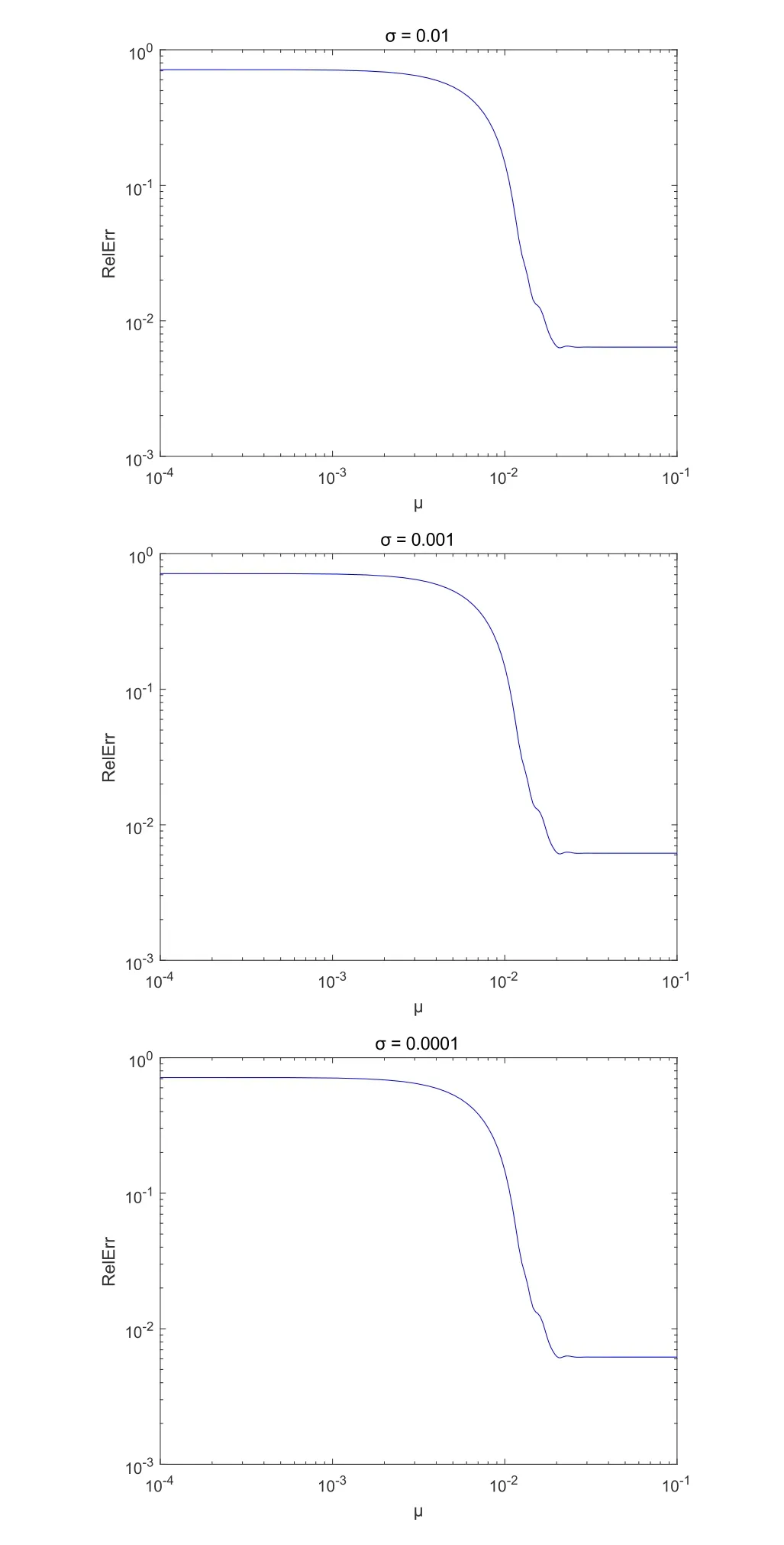
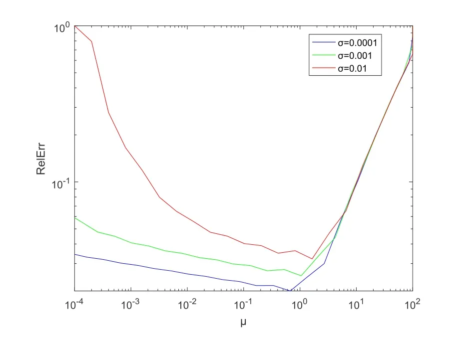
To further illustrate the advantage of the model (3.1),we plot the relative errors for a varying parameterµof models (3.1) and (3.2) in Figures 1 and 2.The horizontal and vertical axes denote the value ofµand relative error“RelErr”,respectively.To avoid repetition,the relative errors of the model (3.1) are plotted in three graphs,which can be seen in the Figure 1.From the Figure 1,we can see that the optimal value ofµfor model (3.1) is almost constant(see the position of minimum in each row).By observing each curve in the Figure 2,it is clear that the optimal value ofµis increased with the noise levelσ.Based on this test,we can conclude that model (3.1) is more stable than model (3.2) with respect to the noise level.

Fig.1 Numerical results of model (3.1) with three noisy cases (m=n=100,r=5,sr=0.5,σ=0.01,0.001,0.0001).

Fig.2 Numerical results of model (3.2) with three noisy cases (m=n=100,r=5,sr=0.5,σ=0.01,0.001,0.0001).

3.2.Nuclear norm and square root least squares problems

In this subsection,we report the efficiency of themethod for solving the problem (1.7) with different experimental settings.Firstly,we test it for solving the problem(1.7) with Gaussian noise.In this test,we choosem=nfrom 100 to 1000 and setsr=0.5,r=5,σ=0.01.The test results are given in the Table 3.From the Table 3,we can clearly see that the model (3.1) is more efficient for high dimensional problems,and a higher accuracy can be obtained compared to the lower dimensional problems.

Table 3 Numerical results of ADMM_NNSR for problem (1.7),m=n,sr=0.5, σ=0.01.

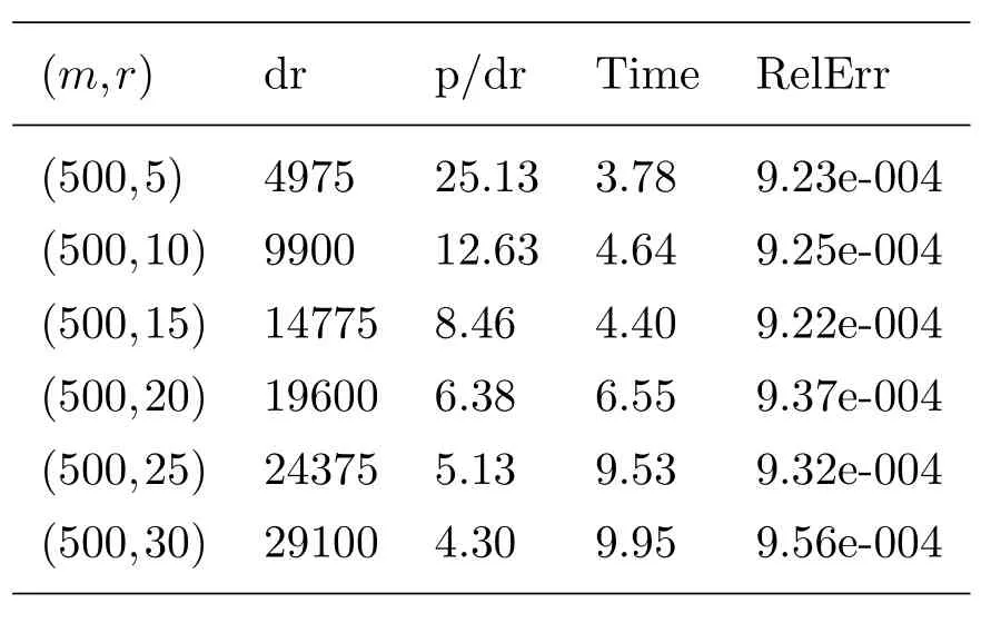
Secondly,we test ADMM_NNSR method asris increasing from 5 to 30.The test results are shown in the Table 4.Observing the Table 4,we can see that the accuracy of the solution is 10−4.In other words,the problem is solved successfully.Moreover,it can be seen from the table that the ADMM_NNSR method needs more time asrincreases except for the caser=15.

Table 4 Numerical results of ADMM_NNSR for problem (1.7) with different r,m=n,sr=0.5

Finally,we test the performance of ADMM_NNSR method for solving problem (1.7) with differentsr.The numerical results can be seen in the Figure 3.From the Figure 3,we can see that as the higher the sampling ratio is,the higher accuracy can be obtained.

Fig.3 ADMM_NNSR for problem (1.7) with Gaussian noise (m=n=500,r=5,sr=0.3,0.5,0.7,0.9, σ=0.01).

§4.Conclusions

In this paper,we first applied the ADMM_NNSR for solving the problem (1.7),which is efficient for solving the high dimensional matrix restoration problem with unknown noise level.The convergence result of the proposed method was given as well.Then we presented some numerical experiments to illustrate the efficiency of the model and the proposed algorithm.Numerical results show that the optimal parameterµdoes not depend on the noise level for the model (3.1),while it needs to be increased withσfor the model (3.2).Furthermore,the model(3.1) is more efficient than model (3.2) in terms of accuracy and running time.Here we devote to illustrating the performance of the ADMM_NNSR for matrix completion problem.In the near future,we will use our proposed method to solve more high-dimensional matrix estimation problems.