The dynamic impact of income and income distribution on food consumption among adults in rural China

LI Lei ,ZHAI Shi-xian,BAI Jun-fei,

1 National Agricultural and Rural Development Research Institute,China Agricultural University,Beijing 100083,P.R.China

2 Beijing Food Safety Policy & Strategy Research Base,Beijing 100083,P.R.China

3 College of Economics and Management,China Agricultural University,Beijing 100083,P.R.China

Abstract Previous studies have demonstrated that income has a significant effect on food demand in rural China. However,little research has focused on the dynamic impact of income and income distribution on food demand in rural China. Using China Health and Nutrition Survey data,this study employs a consistent two-step quadratic almost ideal demand system model,with addressed problems of endogeneity of total expenditure and zero shares,to estimate the food demand elasticities among adults in rural areas with regard to the different income strata. The results show that changes in income and income strata have significant effects on food demand in rural areas. Except for grains,all other food groups,including vegetables,oils and fats,animal products,and other foods,have positive income elasticities,and the rise in the income strata will lead to declining income elasticities for grains,vegetables,oils and fats,and animal products. Based on the estimated income elasticities,the food consumption projections indicate that reducing income inequality in rural society can improve the living standard of low-income people in terms of nutrient intakes.

Keywords:income redistribution,food demand,endogeneity,censored demand system,rural China

1.Introduction

Since China initiated its market-oriented economic reforms in 1978,its growth rate of per capita gross domestic product (GDP) has averaged 7-8% per year.These market-driven reforms have led to a considerable rise in per capita income,also contributed to widening income inequality in rural China. According to the National Bureau of Statistics of China (NBSC),per capita disposable income in rural China grew from 134 CNY in 1978 to 2 246 CNY1Per capita disposable income is deflated by CPI (1978=100).in 2018,or a 16.8-fold increase.Along with the remarkable increase in income,income inequality has been growing in recent decades. According to Sutherland and Yao (2011),the Gini coefficient in rural China rose from 0.21 in 1978 to 0.37 in 2006,displaying a considerable upward trend. Additionally,according to a report by the China Household Finance Survey (CHFS),the Gini coefficient for rural households was 0.60 in 2010,showing an extremely serious income disparity in rural China. Based on China Health and Nutrition Survey(CHNS) data,the Gini coefficients in rural areas were 0.41 in 2004,0.44 in 2006,0.45 in 2009,and 0.43 in 2011,respectively2The Gini coefficients are calculated by the authors using CHNS data from 2004-2011.. A large amount of research in China has been investigating the trends and determinants of income disparities in rural and urban areas as well as the associated impact of income disparities.

However,little research has focused on the dynamic impact of income distribution on food demand in rural China. As disposable income increases and the market develops,consumers tend to shift from staple foods,such as grains,to more expensive food,such as animal products (Huang and Rozelle 1998; Yuanet al.2018). A large number of studies have measured the impact of income on food consumption and its structure in rural China (e.g.,Fanet al.1994,1995; Han and Wahl 1998;Jiang and Davis 2007). Especially need to point out,the aforementioned empirical research assumed that rural residents with different income classes share an identical food consumption structure. While some studies have pointed out that income distribution may result in different food consumption structures (Pinstrup-andersen and Caicedo 1978; Huang and Gale 2009). For instance,the low-income people in rural areas usually spend most of their income on food,and their income can only maintain the basic energy demand.

This study aims to fill out the gap by assessing the dynamic impact of income and income distribution on food consumption in rural China. We particularly focus on rural adults for that the food consumption habits and preferences of this group of people are relatively stable compared to those of children and that adults can obtain and dispose of their own income which directly determines the food quantity consumed. To reach this objective,data from CHNS on rural areas from 2004,2006,2009 and 2011 are used.

In addition,this study extends previous studies from the following two perspectives. First,a consistent twostep quadratic almost ideal demand system (QUAIDS)model,with addressed problems of endogeneity of total expenditure and zero shares,is used to estimate the food demand elasticities with regard to income strata. The almost ideal demand system (AIDS) and QUAIDS models are widely used to measure food demand elasticity with regard to income (expenditure) in studies. However,most of these studies have not addressed the problems related to the endogeneity of total food expenditure variable and zero expenditure shares. In AIDS or QUAIDS model,each food share,the dependent variable,is computed as the ratio of every food category expenditure and total food expenditure. Therefore,the error term may be correlated with total food expenditure variable (Lecocq and Robin 2015). In most empirical studies,some households or individuals consume zero for one or more food categories. Zero consumption has important econometric and economic implications,and statistical estimation procedures that do not account for these zero observations in the dependent variable can lead to biased and inconsistent parameter estimates in demand analysis (Lee and Pitt 1986). Second,we predict the food consumption in rural China by considering the impact of the dynamic changes in the income strata after the variation in income. Studies in literature have attempted to predict the impact of income distribution changes on food consumption in China (e.g.,Zheng and Henneberry 2010; Renet al.2018). The basic conclusion of these studies is that low-income households consume a greater quantity of food than high-income households at the same income growth rate. It should be noted that the above mentioned literature only analyzes from the perspective of static income distribution changes in the prediction,without considering the impact of the dynamic changes in the income strata after the variation in income. For example,when the poorest consumers are no longer in poverty,they may be confronted with different elasticities of food demand,as seen in the higher income groups.Our empirical comparison shows a statistical difference between the projection considering dynamic changes of income strata and the one with static income strata,suggesting a significant bias in the projection with static income strata.

The remainder of this study is organized as follows.Section two presents the empirical demand model addressing the problems of expenditure endogeneity and zero expenditure shares and also describes the data used in this study. Section three displays the empirical demand elasticities and the projected results. Section four presents the discussion about the estimated income elasticities. The final section concludes the findings.

2.Methods and data

2.1.Basic forms of QUAIDS model

The QUAIDS model of Bankset al.(1997),developed on the AIDS model introduced by Deaton and Muellbauer(1980),is a popular task to estimate demand elasticity with regard to price and expenditure (Poi 2012). The QUAIDS model is based on the indirect utility function:

wherexis the expenditure on the goods,anda(p) is price index and is defined as follows:

In the function above,subscriptsiandjindicate goods andpiis the price of goodifori=1,…,n.b(p) is the Cobb-Douglas price aggregator and is defined as follows:

and

Letqirepresent the quantity of goodi,and the expenditure share for goodiisωi=piqi/x. Applying Roy’s identity to eq.(1),the QUAIDS model is given as follows:

whereα0,αi,βi,λi,andγijare parameters to be estimated3In practice,most of researchers,such as Deaton and Muellbauer (1980),Banks et al. (1997),and others,set a fixed value for α0.;uiis the error term. The adding-up,homogeneity,and Slutsky symmetry restrictions on the parameters are as follows:

Demographic variables such as family size and age composition are major determinants of the consumption of food or other commodities (Pollak and Wales 1981). In this study,the QUAIDS model incorporates demographic variables by using the scaling method introduced by Ray(1983) and extended by Poi (2012). Ray’s method adopts the scaling function as follows:

The first termx0(z) means that the expenditure may change as demographic variableszvary. As described by Ray (1983),x0(z) is given as follows:

whereρis a vector of parameters to be estimated.The second termφ(p,z,u) measures the changes in relative prices,and the actual goods may be consumed.Following Poi (2012),φ(p,z,u) is extended as follows:

As in Poi (2012),the QUAIDS model incorporating demographic variables is given as follows:

The price and expenditure elasticities from eq.(6) are given by Poi (2012). The uncompensated (Marshallian)price elasticity of goodiwith respect to pricejis denoted by the following:

where Δijis the Kronecker delta,which equals one wheni=j; otherwise Δij=0. The expenditure elasticity for goodiis given as follows:

The compensated (Hicksian) price elasticity can be calculated from the Slutsky equation:

2.2.Handling endogenous expenditure and zero expenditure shares

In the food demand system,each food category share is computed by dividing total-budget expenditure by the expenditure of each good item. In each share equation,the error termuiin eq.(6) may be correlated with the total expenditure term lnx. Therefore,the total expenditure term lnxand (lnx)2in the QUAIDS model may be endogenous (Blundell and Robin 1999). To address the problem of endogeneity of expenditure terms,an augmented regression specification,as Blundell and Robin (1999) suggested,is used to test and rectify the endogeneity of lnxand (lnx)2. The first step of the procedure is to predict the residual termfrom a reduced-form equation for lnx=Mτ+v,whereM,a matrix form andM=[1,lny,(lny)2,lnp,z],consists of a set of explanatory variables including income,prices of goods consumed,and demographic variables that are the same as those in eq.(6),andτis a vector of parameters to be estimated. The residual termis written into eq.(6) as the orthogonal decomposition:

andE(εi|M,υ) is assumed for alli. The adding-up property requires,and the significance of parameterθiis a direct test of the endogeneity of the expenditure terms lnxand (lnx)2.

When data used in food demand systems are not censored or complete,the parameters in the demand equations may be consistently and efficiently estimated by iterative seemingly unrelated regressions (SUR) or maximum likelihood (ML). However,if some households or individuals do not consume all food items,the problem of censoring data arises. If the data used in food demand are collected in a short period,for example,in a weak period,it is likely to observe zero expenditure shares for certain food items. Ignoring zero expenditure shares may cause biased and inconsistent estimators (Lee and Pitt 1986).

To address the problem of zero observations,the consistent two-step (CTS) estimation procedure introduced by Shonkwiler and Yen (1999) was used for demand systems of censored dependent variables. According to Shonkwiler and Yen (1999),the unconditional mean of theith food group expenditure shareωican be denoted as follows:

wheref(xi,β) represents the deterministic component of eq.(6),which is nonlinear inβ; Φ(zi´δ) is the univariate standard normal cumulative distribution function (CDF),andφ(zi´δ) is the univariate standard normal probability density function (PDF).

Using eq.(11) combined with eq.(6),the demand system of equations can be rewritten as follows:

whereui=ωi-E(ωi|xi,zi). The demand system of eq.(12)can be estimated by the CTS procedure. The first step of the CTS is to obtain probit model estimatesofδwith ML. The second step consists of calculatingandand using a nonlinear SUR model to estimateβandσiin the following equation:

In the eq.(13),uishould be written as follows:

whereεiis the random error term. Since the ML probit estimator vectoris consistent,the second step of applying SUR estimation also obtains consistent (though inefficient) estimators. However,the error termsuiin eq.(13)are heteroskedastic,and therefore,the covariance matrix of the second-step estimator is incorrect (Shonkwiler and Yen 1999). To address this problem,we use a bootstrap method for the parameters and obtain efficient estimators(as well as a correct covariance matrix).

Because of adding-up restrictions,the corresponding covariance matrices in demand systems are generally singular. However,when accounting for zero expenditure shares,the demand system in eq.(13) may violate adding-up restrictions (Shonkwiler and Yen 1999; Yenet al.2002). To account for the adding-up property in the demand system above,we follow Yenet al.(2003) and estimate the firstn-1 goods,with thenth good chosen as a residual category (also see,Yen and Lin 2006; Zheng and Henneberry 2010).

When using the CTS procedure to address zero food expenditure shares in the QUAIDS model,the formulas for the price elasticity need to be rewritten as follows:

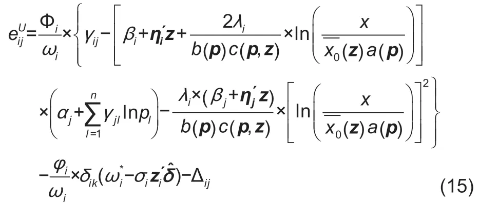
whereδikrepresents the parameter of the logarithm price used in the probit model. The expenditure also needs to be adjusted as follows:

The compensated (Hicksian) price elasticity can be calculated from eq.(9).

As we predict the impact of income and income distribution on food demand,income elasticity for foodiis needed. The food expenditure function is given as follows:

where lnxis the logarithm form of total food expenditure,lnyis the logarithm form of consumer income,zrepresents a vector of demographic variables that may affect food expenditure,andTandDrepresent time and district variables,respectively. The income elasticity with regard to food expenditurexisex=b1+2b2lny,and the income elasticity with respect to theith food quantity consumed can be calculated by the following equation:

To simulate the dynamic impact of income redistribution,the computed income elasticities are used to project the demand for each food item based on the different hypotheses of changing income and income distribution.Before performing projections for food demand,several assumptions suggested by Zheng and Henneberry(2010) are needed. First,the adults’ preferences and the prices of food groups are assumed to be unchanged for each income stratum. Second,market development and urbanization,which may affect food demand,are not considered. Finally,the population size of each income stratum,unlike Zheng and Henneberry (2010) and Renet al.(2018),is assumed to vary dynamically with the changes in income and income distribution. That is,the change in food demand depends on the change in income and income distribution as well as the change in population size in each stratum. The simulated impact of changed income,income distribution,and population size on the quantity of each food group in every income stratum is given as follows:

where ΔQi(d)represents the change in the total quantity consumed of theith food group in thedth income stratum,(Δy/y)ddenotes the change in income in thedth income stratum,andEy,i(d)is the income elasticity for theith food group indth stratum.is the average daily consumption quantity of food groupifor each adult individual;Ndis the sample size of all the adults in thedth stratum.

2.3.Data

The data used for our study come from the CHNS. These data are jointly collected by the Carolina Population Center at the University of North Carolina at Chapel Hill and the National Institute for Nutrition and Health at the Chinese Center for Disease Control and Prevention.The CHNS database is designed for the study of issues related to health and nutrition in China through a multistage and random cluster process to draw a sample of representative individuals and households. Data on household food consumption were collected randomly for three consecutive days in a weak. In addition to household food consumption data,detailed individual dietary intake (24-h recall),both away from home and at home for the same three consecutive days,were also collected for all family members. The CHNS has been conducted more than nine rounds since 1989,and until 2011,this survey was conducted for nine rounds.

To reflect the impact of income distribution in the new era,the CHNS data from 2004,2006,2009,and 2011 are used in this study to investigate food demand in rural China. Because the individual food consumption both away from home and at home in the CHNS data can show the entire dietary intake for an individual,we limit our sample to adults aged 18 and above in rural areas.We dropped the observations with missing values for the dependent and independent variables used in eq.(13),as well as the observations with a yearly income below 100 CNY,which is too low to survive even in poor areas of rural China. Additionally,we deleted the observations of adults who are still in school,as well as those of pregnant women in rural areas. Ultimately,a total of 10 780 observations were used in this study.

Referring to Jiang and Davis (2007),the food groups used in this study consist of five food categories in rural areas:grains,vegetables,oils and fats,animal products(including eggs,meat,aquatic products and dairy products) and other foods. Considering the absence of individual oil and fat consumption data,we use household per capita oil and fat consumption data to represent individual-level data. The dependent variable is the average quantity of each food group consumed daily,and the key explanatory variables in this study are the income and price variables. Using the quantities and prices of food groups,we can obtain each food group expenditure share and total food expenditure in this study.

An adult’s food consumption is affected not only by individual income but also by household income. Based on the work of Mao and Yao (2015),a new individual income in this study is computed as follows. First,we calculate the residual household income (household total income minus all the household members’ wage income). Second,we divide the residual household income by the household size,plus individual income,and obtain a newly constructed yearly individual income.Given the average daily food consumption data for this study,we use a real average daily income4Dividing a constructed yearly income by 360 days equals to an average daily income,and then deflating it by CPI with 2004 as the base year results in the real average daily income.to investigate the impact of income distribution on food consumption in rural China.

There are many studies of food demand that use unit prices (expenditures divided by the quantity consumed),rather than actual prices in the market,which may cause analysis bias because unit values are not exogenous (Yu and Abler 2009). Using the market price may be helpful in addressing the endogeneity of the unit price. In our study,we employ free market price for each food item at the community level,sourced from the Carolina Population Center at the University of North Carolina,to analyze the impact of price on food demand in rural China. Accroding to Khanalet al.(2016),the value-weighted price of each food group can be calculated from the following equation:

Taking a deflated price5Deflating the value-weighted price by CPI with 2004 as the base year results in a deflated price of each food group.as each food group price,food expenditure can be calculated by food quantity consumed with each food group price. Aggregating all five food group expenditures turns out to be total food expenditure in the QUAIDS model.

The demographic variables (gender,age,education level,marital status,and so on) that may have effects on food demand and nutrient intake (Kroshus 2008; Liuet al.2015; Renet al.2019; Zhao and Zheng 2019). In this study,the demographics,including gender,age,marital status,education year,household size,year and district variables,are controlled in the QUAIDS model. All the definitions of independent variables are displayed in Table 1. Except for income,expenditure,price,education year,and household size variables,which are continuous variables,the remaining variables in the QUAIDS model are set as dummy variables.

In this study,all the individual samples are equally segmented into seven income strata (ranging from the lowest level to the highest level) based on average daily income. Table 2 gives the descriptive statistics about daily average food quantities,prices,expenditure and individual income among different income strata. The average quantity consumed for grains,vegetables,and oils and fats are similar across income groups,while the average quantity consumed for animal products and other foods maintain a clear growth trend,with the change in income strata from the lowest to the highest level.There are very large differences in mean income among the seven income strata when low-income groups are compared to high-income groups. For example,the mean income in the highest income strata is more than 18 times that in the lowest income strata.

Table 3 presents descriptive statistics about demographic variables that may affect food demand in rural China. Compared to high-income groups,adults in low-income groups have lower education levels and larger family sizes.

3.Results

Not all the individuals consumed all the food groups in this study,and the ratios of zero expenditure shares for grains,vegetables,oils and fats,animal products,and other foods are 0.01,0.23,2.37,12.74,and 34.74%,respectively.Since the percentage of zero expenditure shares in grains and vegetables are quite low (less than 1%),we only use the CTS procedure introduced by Shonkwiler and Yen(1999) to address the zero problem in the remaining food groups (oils and fats,animal products,and other foods).As noted before,we treat the last food group (other foods)as the residual food category. Applying the properties of adding-up,homogeneity,and Slutsky symmetry,we can obtain all the coefficients of the last food group equation.

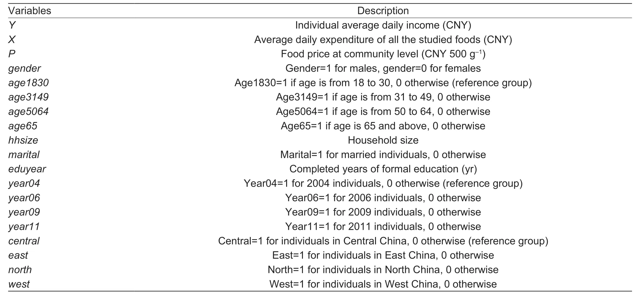
Table 1 Definitions of independent variables regarding food demand in rural China

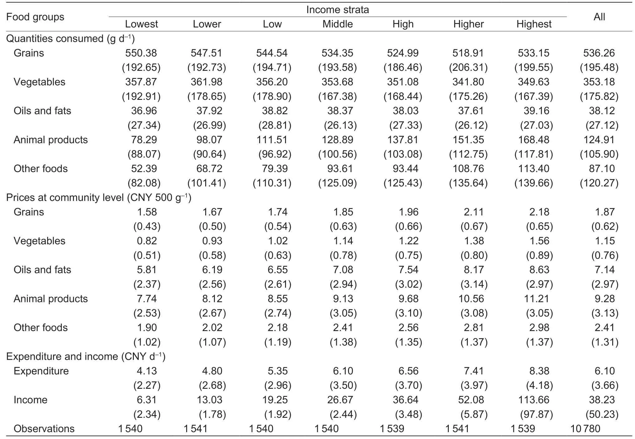
Table 2 Descriptive statistics of food quantities,prices,expenditure and individual income

The QUAIDS model contains the AIDS model under the joint hypothesis ofλi=0,fori=1,…,m. As shown in Appendix A,the parameters of the squared logarithm of food expenditure (λi) are all significantly different from 0.This suggests that the QUAIDS model meets the needs of this study. To address the endogeneity of the QUAIDS model in this study,the method suggested by Blundell and Robin (1999) is used to test and rectify the exogeneity of expenditure terms lnxand (lnx)2. The results show that the null hypothesis of exogeneity of expenditure terms is rejected for all the food groups at the 5% significant level(Appendix A) and verify that the method has rectified the endogeneity of the expenditure terms.

3.1.Elasticities

After all the coefficients in eq.(13) are obtained,we can use the elasticity formats in eqs.(9),(15) and (16) and the sample means of explanatory variables to calculate the Marshallian own price,the Hicksian own price and the expenditure elasticity of all the food groups. To obtain income elasticity,we use the OLS method to estimate the parameters in eq.(17) and calculate the income elasticity of all food groups using the elasticity format in eq.(18).

To evaluate the confidence of own price,food expenditure,and income elasticities,the elasticity bootstrapping method introduced by Krinsky and Robb(1986) is used to evaluate the confidence of own price,food expenditure and income elasticities,estimating whether each elasticity is significantly different from 0.The Marshallian (uncompensated) own price,Hicksian(compensated) own price,food expenditure and income elasticities for five studied food groups are shown in Table 4. The estimated income elasticities at sample mean with regard to food expenditure are 0.156,0.150,0.147,0.145,0.143,0.140,and 0.136 from the lowest to highest income stratum,respectively. For the whole sample,the income elasticity with respect to food expenditure is 0.145,and all of these elasticities are significantly different from zero at the 1% level.

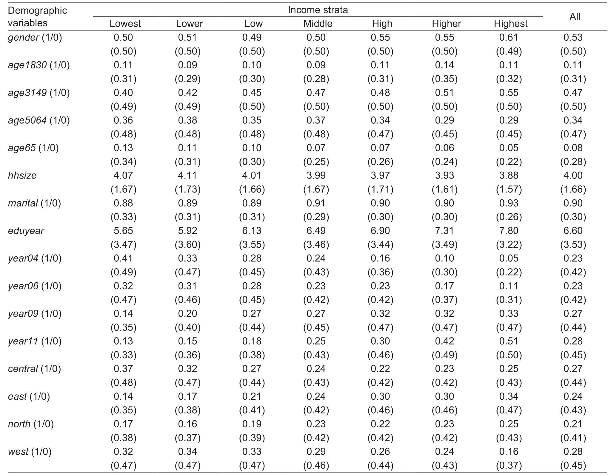
Table 3 Descriptive statistics of demographic variables

As shown in Table 4,all price elasticities are negative and most of them are statistically significant at the 5%level for the seven income strata. For income elasticity,with the exception of grains,the other four food item income elasticities are all positive and statistically significant at the 1% level,which shows that the other food groups are normal goods for rural adults.

The estimated income elasticities are below 1 for all five food groups,and they maintain a downward trend as the income grows. For example,the animal product income elasticity is 0.400 in the lowest income stratum but declines to 0.293 in the highest income stratum. In particular,for grains,income elasticities at high-income levels are close to or even below 0. This indicates that the grain group is an inferior goods group at high-level income strata. This finding is similar to that of Huang and Gale (2009).

3.2.Projection

To reach the simulated results,the estimated impact of dynamic income redistribution on food demand in rural areas is presented in this section. Three ways of changing current income distribution are considered:(1)increasing the incomes of all the income strata at the same growth rate; (2) increasing the incomes of the lowlevel income strata; (3) transferring incomes from highlevel income strata to low-level income strata. The three ways of income redistribution consist of six scenarios,each scenario simulates the impacts of the change in income and income distribution on food demand among adults in rural China. Based on the work of Pinstrupandersen and Caicedo (1978),1% of the total income of all adults is set as the amount of change in each scenario(Zheng and Henneberry 2010; Renet al.2018). Unlikestatic simulation of aforementioned studies,we adopt a 1% change in total income under the dynamic population size in income strata to simulate the change in food consumption as well as compare it with the simulated food consumption under the static population size hypothesis.

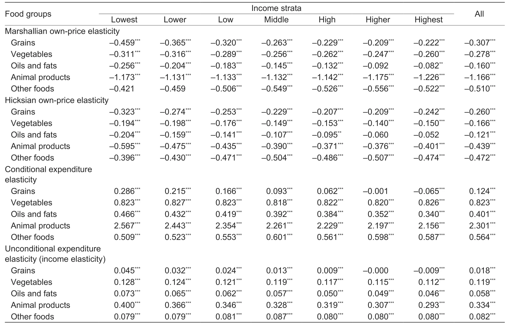
Table 4 Own-price,expenditure,and income elasticities for food consumed in rural China

The six projection scenarios are presented in Table 5. Scenario one,with regard to the first way of income redistribution,increases all seven income strata at the same rate,in which the population sizes in the seven income strata are in a variation of -27,-30,4,4,14,-1,and 36 from the lowest to the highest strata,respectively. Scenarios two to four,with regard to the second way of income redistribution,involve increasing the incomes of the low-income strata. Scenario two increases the incomes of the lowest and lower strata,in which 667 adults are in varied income strata from the lowest to lower income stratum,and the other five do not vary in their observations. Scenario three,increases the incomes of those in the lowest and lower strata at the same rate,in which the population sizes of the three low-income groups are in a variation of -294,-197,and 491; the others do not change. Scenario four increases the incomes of the lowest,lower,and low strata at the same rate,in which the population size from the lowest to the middle income strata are in a variation of-167,-108,-53,and 328; the others do not change.Scenarios 5 and 6,with regard to the third way of income redistribution,involve redistributing current incomes from high-income to low-income strata. Scenario 5 transfers the incomes from the highest to the lowest income strata,with 667 adults rising from the lowest to the lower income strata and 82 adults dropping from the highest to the higher income strata. Scenario 6 transfers the incomes from the highest stratum to the lowest stratum and from the higher stratum to the lower stratum at the same rate. In this scenario,the population sizes in the seven strata are in a variation of -294,-197,491,0,81,-28,and -53 from the lowest to the highest stratum,respectively.

The projection of income distribution and observations under the six different hypotheses is presented in Table 5.As we can see,even if each income stratum maintains a 1% increase in income,the sample size of each income class also changes slightly. Apparently,if the selected 1% in total population income only increases in the lowest income stratum (scenarios 1 and 5),the new samplesize,as well as the income share,changes obviously compared with the current sample size. Taking scenario 5 as an example,1% of the total population income is transferred from the highest to lowest income stratum,contributing to the drop in the sample sizes in the lowest stratum from 1 540 to 873 and in the highest stratum from 1 539 to 1 457,as well as the decrease in the income shares in the lowest strata from 2.359 to 1.401% and in the highest stratum from 42.448 to 40.208%. As the main focus of this study is to detect food demand for alternative income distribution patterns,a small change in income distribution patterns may lead to a remarkable variation in food demand.

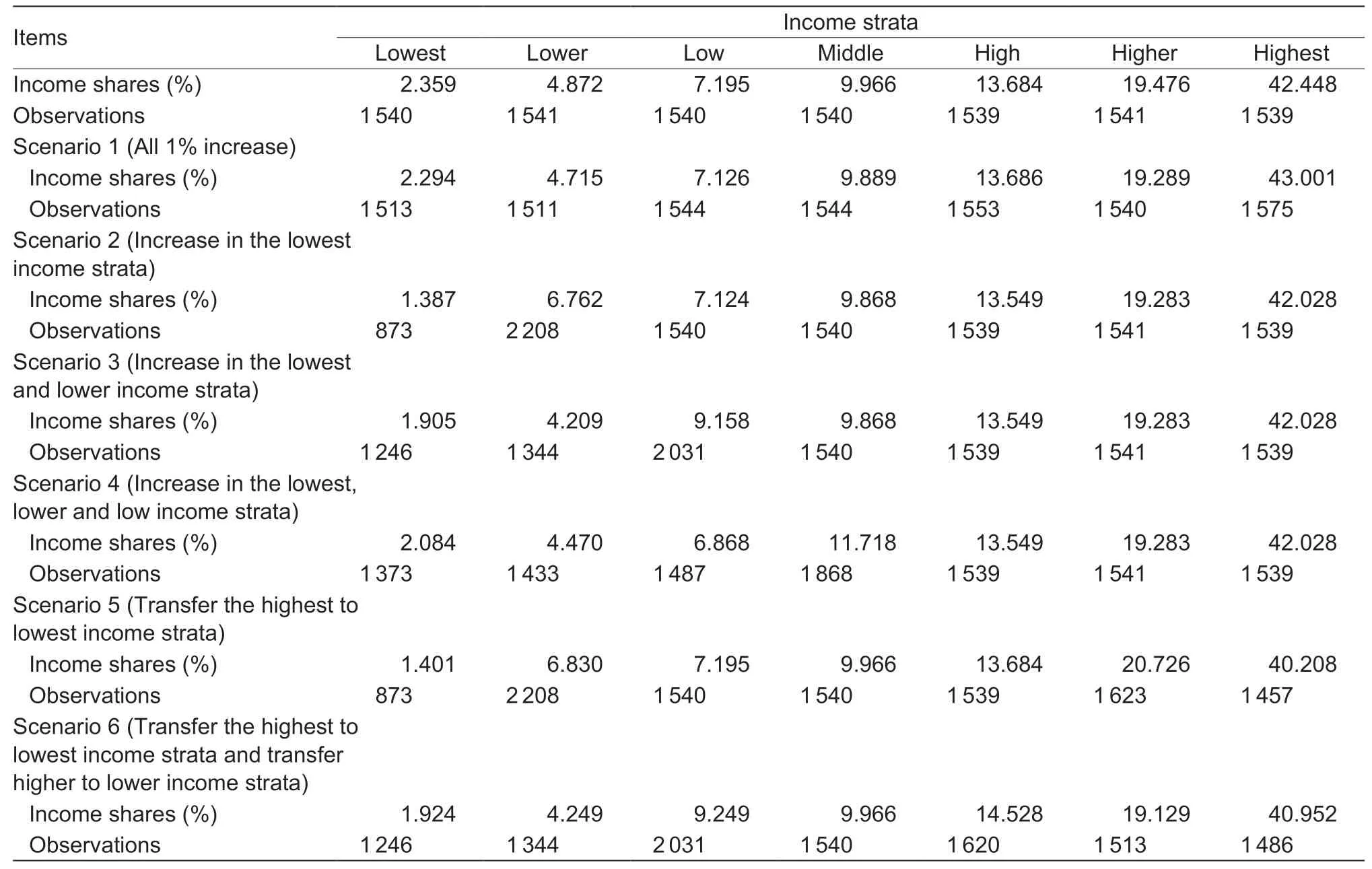
Table 5 Estimated income distribution on food demand based on six scenarios in rural China

Based on eq.(19),the simulation changes in food demand among adults in rural China based on the six scenarios mentioned above are presented in Table 6.

Compared with the current food consumption,the food quantity consumed due to a unified 1% increase in total income in each income stratum is still rising (Table 6,column 4). However,despite a slight change in the population size and income distribution of each income stratum based on both dynamic and static hypotheses in scenario one,there is little difference in changes in food demand between the dynamic and static hypotheses.From scenarios two to four,the simulated food growth rate maintains a downward trend from 0.551 to 0.273%(Table 6,row 13),as a result of the 1% increase in total population income from only one income stratum (the lowest income group) to three low-income strata (the lowest,lower,and low group). From two redistribution scenarios (scenarios 5 and 6),we can see that redistribution will increase food consumption even if the total income does not increase. Compared the static(population unchanged at all income strata) and dynamic(population size in each income stratum varying with income) results,simulated food demand under static observation in each group tends to be overestimated.

4.Discussion

The estimated results indicate that income elasticities differ in various food groups. Similar as meta-analysis results by Zhouet al.(2020),animal products have higher income elasticities than necessities such as grain products. Table 4 shows that the income elasticities of all the observations are 0.018 for grains,0.119 for vegetables,0.058 for oils and fats,0.334 for animal products,and 0.082 for other foods. These elasticitiessuggests that rural residents tend to consume more animal products than grain products as their income increases.

Table 6 Estimated increase in food demand based on income distribution and sample size in rural China

Income elasticities for the same food category vary across income strata. The consumers in low-income strata are more sensitive to income change for the moststudied food groups than those in high-income strata. For example,with the rise in the income strata,the income elasticity of food gradually decreases. More specifically,in the higher and highest income groups,income elasticity began to gradually drop below zero,and grains began to become “inferior goods”.

As the income increases,the income distribution may also change. When we project the impact of income growth,the dynamic changes in the income strata need to be considered. Studies in literature such as Zheng and Henneberry (2010) and Renet al.(2018) predicted the impact of income distribution changes on food consumption in China,but their analyses were both based on static income distribution in the prediction,without considering the impact of the dynamic changes in the income strata after the growth in income. As shown in Table 5,when the income rises,compared to static scenario,the population size in each income group varied under the dynamic case. Table 6 shows that the food demand in the future may be overestimated if the dynamic of income distribution is neglected.

5.Conclusion

In this study,we investigate the impact of income distribution on food demand among adults in rural China.To reach this goal,two steps are conducted. First,the food demand elasticities in rural China are estimated by income strata using an individual food consumption data source from the CHNS (2004-2011). Second,the estimated income elasticities of studied food groups for different income strata are then used to simulate the response of food consumption with the changes in incomes and income distribution under six scenarios.The major findings with regard to the impact of income distribution on food demand among adults are described below.

First,for income elasticity,with the exception of grains,the other four foods income elasticities are all positive and statistically significant at the 1% level,which shows that the other food groups are normal goods for rural adults.In particular,for grains,income elasticities are close to or even below 0 at high-income levels,indicating that grains are becoming inferior goods.

Second,changes in both income and income distribution have significant effects on food demand across the seven income strata under the six scenarios.The results indicate that when the variation in the population size of each income stratum is ignored,the simulation of food demand may be overestimated. The hypothesis of dynamic change in population size in each income stratum would show more reasonable projected food demand than those of static constant population size.

Finally,the projected results indicate that both raising the income of low-income people and transferring from high-income groups to low-income people can help improve the nutrition and living standard of the lowincome population. Reducing income inequality,such as subsidizing low-income people,could improve the living standard of the low-income population,while not hurt high-income population in terms of nutrient intakes.

Acknowledgements

The authors acknowledged the support from the National Natural Science Foundation of China (71673316) and Beijing Food Safety Policy & Strategy Research Base,China. This research uses data from the China Health and Nutrition Survey (CHNS). We are also grateful to research grant funding from the following sources:the National Institutes of Health (NIH) and the Eunice Kennedy Shriver National Institute of Child Health and Human Development (NICHD) for R01 HD30880; the National Institute of Diabetes and Digestive and Kidney Diseases (NIDDK) for R01DK104371 and R01HL 108427;the NIH Fogarty Grant D43 TW009077 for financial support for the CHNS data collection and analysis files since 1989; the China-Japan Friendship Hospital,Ministry of Health,for support for the CHNS 2009; the Chinese National Human Genome Center at Shanghai since 2009;and the Beijing Municipal Centers for Disease Prevention and Control since 2011. We are also grateful for funding from the NICHD to the Carolina Population Center at the University of North Carolina at Chapel Hill (NIH Grant;P2C HD050924 and T32 HD007168).

Appendixassociated with this paper can be available on http://www.ChinaAgriSci.com/V2/En/appendix.htm