End-to-end differentiable learning of turbulence models from indirect observations

Carlos A.Michelén Ströfer ,Heng Xiao

Kevin T. Crofton Department of Aerospace and Ocean Engineering, Virginia Tech, Blacksburg, Virginia, United States

ABSTRACT The emerging push of the differentiable programming paradigm in scientific computing is conducive to training deep learning turbulence models using indirect observations.This paper demonstrates the viability of this approach and presents an end-to-end differentiable framework for training deep neural networks to learn eddy viscosity models from indirect observations derived from the velocity and pressure fields.The framework consists of a Reynolds-averaged Navier–Stokes (RANS) solver and a neuralnetwork-represented turbulence model,each accompanied by its derivative computations.For computing the sensitivities of the indirect observations to the Reynolds stress field,we use the continuous adjoint equations for the RANS equations,while the gradient of the neural network is obtained via its built-in automatic differentiation capability.We demonstrate the ability of this approach to learn the true underlying turbulence closure when one exists by training models using synthetic velocity data from linear and nonlinear closures.We also train a linear eddy viscosity model using synthetic velocity measurements from direct numerical simulations of the Navier–Stokes equations for which no true underlying linear closure exists.The trained deep-neural-network turbulence model showed predictive capability on similar flows.

Key words:Turbulence modeling Machine learning Adjoint solver Reynolds-averaged Navier-Stokes equations

There still is a practical need for improved closure models for the Reynolds-averaged Navier–Stokes (RANS) equations.Currently,the most widely used turbulence models are linear eddy viscosity models (LEVM),which presume the Reynolds stress is proportional to the mean strain rate.Although widely used,LEVM do not provide accurate predictions in many flows of practical interest,including the inability to predict secondary flows in noncircular ducts [1] .Alternatively,non-linear eddy viscosity models(NLEVM) capture nonlinear relations from both the strain and rotation rate tensors.NLEVM,however,do not result in consistent improvement over LEVM and can suffer from poor convergence [2] .Data-driven turbulence models are an emerging alternative to traditional single-point closures.Data-driven NLEVM use the integrity basis representation [3,4] to learn the mapping from the velocity gradient field to the normalised Reynolds stress anisotropy field,and retain the transport equations for turbulence quantities from a traditional model.

It has been natural to train such models using Reynolds stress data [4,5].However,Reynolds stress data from high-fidelity simulations,i.e.from direct numerical simulations (DNS) of the Navier–Stokes equations,is mostly limited to simple geometries and low Reynolds number.It is therefore desirable to train withindirect observations,such as quantities based on the velocity or pressure fields,for which experimental data is available for a much wider range of complex flows.Such measurements include full field data,e.g.from particle image velocimetry,sparse point measurements such as from pressure probes,and integral quantities such as lift and drag.Training with indirect observations has the additional advantage of circumventing the need to extract turbulence scales that are consistent with the RANS modelled scales from the high fidelity data [5] .

Recently,Zhao et al.[6] learned a zonal turbulence model for the wake-mixing regions in turbomachines in symbolic form (e.g.,polynomials and logarithms) from indirect observation data by using genetic algorithms.Similarly,Saïdi et al.[7] learned symbolic algebraic Reynolds stress models generalisable for two-dimensional separated flows.However,while symbolic models are easier to interpret,they may have limited expressive power as compared to,for instance,deep neural networks [8],which are successive composition of nonlinear functions.Symbolic models may therefore not be generalisable and be limited to zonal approaches.More importantly,gradient-free optimisation method such as genetic programming may not be as efficient as gradient-descent methods,and the latter should be used whenever available [9].In particular,deep learning methods [10] have achieved remarkable success in many fields and represent a promising approach for data-driven NLEVM[4].

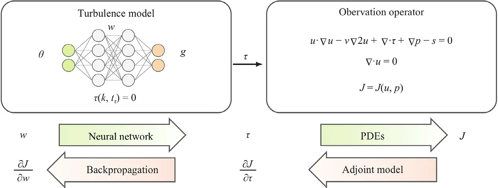
Fig.1.Schematic of the end-to-end differentiable training framework.The framework consists of two main components,the turbulence model and the observation operator,each of which has a forward and backwards (adjoint) model.For any value of the trainable parameters w the gradient of the objective function J can be obtained by solving these four problems.The turbulence model consists of a deep neural network representing the closure function using the integrity basis representation θ g and transport equations T(k,tτ)=0 for the turbulence quantities.The observation operator consists of solving the RANS equations with the proposed turbulence model and extracting the quantities of interest that are compared to the observations in the cost function J.

A major obstacle for gradient-based learning from indirect observations is that a RANS solver must be involved in the training and the RANS sensitivites are required to learn the model.While,such sensitivites can be obtained by using adjoint equations,which have long been used in aerodynamic shape optimisation [11],these are not generally rapidly available or straight forward to implement.The emerging interest in differentiable programming is resulting in efficient methods to develop adjoint accompanying physical models,including modern programming languages that come with built-in automatic differentiation [12],or neural-networkbased solutions of partial differential equations [13].Recently,Holland et al.[14] used the discrete adjoint to learn a corrective scalar multiplicative field in the production term of the Spalart–Allmaras transport model.This is based on an alternative approach to data-driven turbulence modeling [15] in which empirical correction terms for the turbulence transport equations are learned while retaining a traditional linear closure (LEVM).In this work we demonstrate the viability of training deep neural networks to learn general eddy viscosity closures (NLEVM) using indirect observations.We embed a neural-network-represented turbulence model into a RANS solver using the integrity basis representation,and as a proof of concept we use the continuous adjoint equations to obtain the required RANS sensitivities.This leads to an end-toend differentiable framework that provides the gradient information needed to learn turbulence models from indirect observations.

It is worth noting that the intrinsic connection between neural networks and adjoint differential equation solvers has long been recognized in the applied mathematics community [16,17].Recent works have explored this idea in learning constitutive or closure models in computational mechanics [18],in non-Newtonian fluid mechanics [19] and specifically in turbulence flows [20,21].However,note that the representation of turbulent stress in [20] lacked tensorial consistency.

Differentiable framework for learning turbulence models

In this proposed framework a neural network is trained by optimising an objective function that depends on quantities derived from the network’s outputs rather than on those outputs directly.The training framework is illustrated schematically in Fig.1 and consists of two components:the turbulence model and the objective function.Each of these two components has aforwardmodel that propagates inputs to outputs and abackwardsmodel that provides the derivatives of the outputs with respect to the inputs or parameters.The gradient of the objective functionJwith respect to the network’s trainable parameterswis obtained by combining the derivative information from the two components through the chain rule as

whereτis the Reynolds stress tensor predicted by the turbulence model.

Forward Model

For given values of the trainable parametersw,the forward model evaluates the cost functionJ,which is the discrepancy between predicted and observed quantities.The forward evaluation consists of two main components:(i) evaluating the neural network turbulence model and (ii) mapping the network’s outputs to observation space by first solving the incompressible RANS equations.

The turbulence model,shown on the left box in Fig.1,maps the velocity gradient field to the Reynolds stress field.The integrity basis representation for a general eddy viscosity model [3] is given as

whereais the anisotropic (deviatoric) component of the Reynolds stress,bis the normalised anisotropic Reynolds stress,Tandθare the basis tensor functions and scalar invariants of the input tensors,gare the scalar coefficient functions to be learned,andIis the second rank identity tensor.The input tensors are the symmetric and antisymmetric components of the normalised velocity gradient:S=andR=wheretτis the turbulence time-scale anduis the mean velocity.The linear and quadratic terms in the integrity basis representation are given as

where curly braces {·} indicate the tensor trace.

Different eddy viscosity models differ in the form of the scalar coefficient functionsθgand in the models for the two turbulence scale quantitieskandtτ.We represent the scalar coeffi-cient functions using a deep neural network with 10 hidden layers with 10 neurons each and a rectified linear unit (ReLU) activation function.The turbulence scaling parameters are modelled using traditional transport equationsT(k,tτ)=0 with the TKE production termPmodified to account for the expanded formulation of Reynolds stress:P=τ:∇u,where:denotes double contraction of tensors.

The RANS solver along with its post-processing serves as an observation operator that maps the turbulence model’s outputs(Reynolds stressτ) to the observation quantities (e.g.,sparse velocity measurement,drag).This is shown in the right box in Fig.1.The first step in this operation is to solve the RANS equations with the given Reynolds stress closure to obtain mean velocityuand pressurepfields.This is followed by post-processing to obtain the observation quantities (e.g.,sampling velocities at certain locations or integrating surface pressure to obtain drag).When solving the RANS equations,explicit treatment of the divergence of Reynolds stress can make the RANS equations ill-conditioned [22,23].We treat part of the linear term implicitly by use of an effective viscosityνeffwhich is easily obtained since with the integrity basis representation the linear term is learned independently.The incompressible RANS equations are then given as

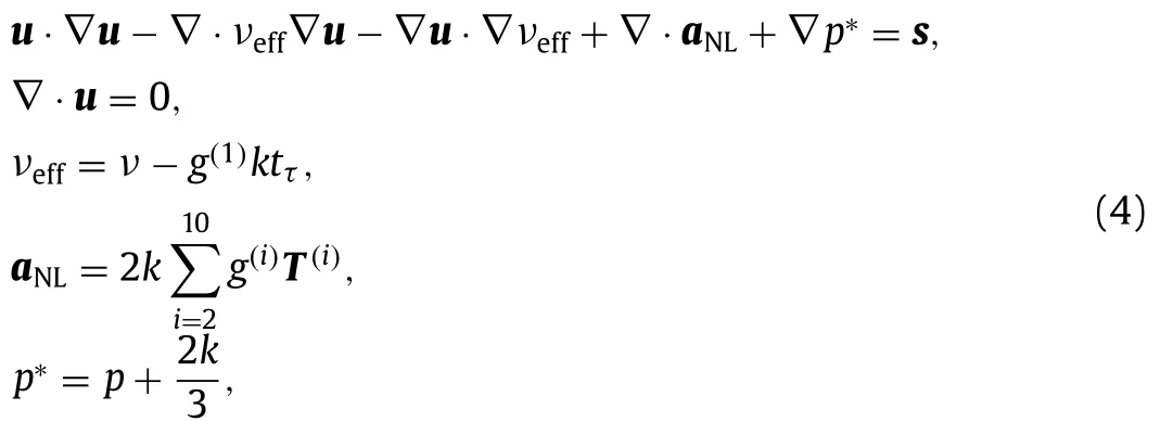
where the term ∇·νeff∇uis treated implicitly.HereaNLrepresents the non-linear component of the Reynolds stress anisotropy,the isotropic component of Reynolds stress is incorporated into the pressure termp∗,andsis the momentum source term representing any external body forces.The coefficientsg(i)are outputs of the neural network-based turbulence model that have the fieldsθas input.

Adjoint Model

For a proposed value of the trainable parameterswthe backwards model (represented by left-pointing arrows in Fig.1) provides the gradient∂J/∂wof the cost function with respect to the trainable parameters.This is done by separately obtaining the two terms on the right hand side of Eq.(1):(i) the gradient of the Reynolds stress∂τ/∂wfrom the neural network turbulence model and (ii) the sensitivity∂J/∂τof the cost function to the Reynolds stress,using their respective adjoint models.Combining the two adjoint models results in an end-to-end differentiable framework,whereby the gradient of observation quantities (e.g.sparse velocity) with respect to the neural network’s parameters can be obtained.

The gradient of the Reynolds stress with respect to the neural network’s parameterswis obtained in two parts using the chain rule.The gradient of the neural network’s outputs with respect to its parameters,∂g/∂w,is efficiently obtained by backpropagation,which is a reverse accumulation automatic differentiation algorithm for deep neural networks that applies the chain rule on a per-layer basis.The sensitivities of the Reynolds stress to the coefficient functions are obtained asfrom differentiation of Eq.(2),which is a linear tensor equation.

For the sensitivity of the objective function with respect to the Reynolds stress we derived the appropriate continuous adjoint equations (Appendix A).Since the Reynolds stress must satisfy the RANS equations,this is a constrained optimisation problem.The problem is reformulated as the optimisation of an unconstrained Lagrangian function with the Lagrange multipliers described by the adjoint equations.The resulting adjoint equations are

For interested readers,Appendix A presents the derivation of the continuous adjoint equations,while Appendix B shows how to use this approach for different types of experimental measurements.Specifically,Appendix B shows how to express different objectives functions as integrals over the domain and boundary,as required by the adjoint equations.Additional details can also be found in Ref.[27].

Gradient Descent Procedure

The training is done using the Adam algorithm,a gradient descent algorithm with momentum and adaptive gradients commonly used in training deep neural networks.The default values for the Adam algorithm are used,including a learning rate of 0.001.The training requires solving the RANS equations at each training step.In a given training step the inputsθiare updated based on the previous RANS solution and scaled to the range 0-1,and the RANS equations are then solved with fixed values for the coefficient functionsg.The inputsθiand their scaling parameters are fixed at a given training step and converge alongside the main optimisation of the trainable parametersw.

Initialisation of the neural network’s parameters requires special consideration.The usual practice of random initialisation of the weights is not suitable in this case since it leads to divergence of the RANS solution.We use existing closures (e.g.a laminar model withg(i)=0 or a linear model withg(1)=−0.09) to generate data for pre-training the neural network and thus provide a suitable initialisation.This has the additional benefit of embedding existing insight into the training by choosing an informed initial point in the parameter space.When pre-training to constant values (e.g.g(1)=−0.09) we add noise to the pre-training data,since starting from very accurate constant values can make the network difficult to train.

Test cases

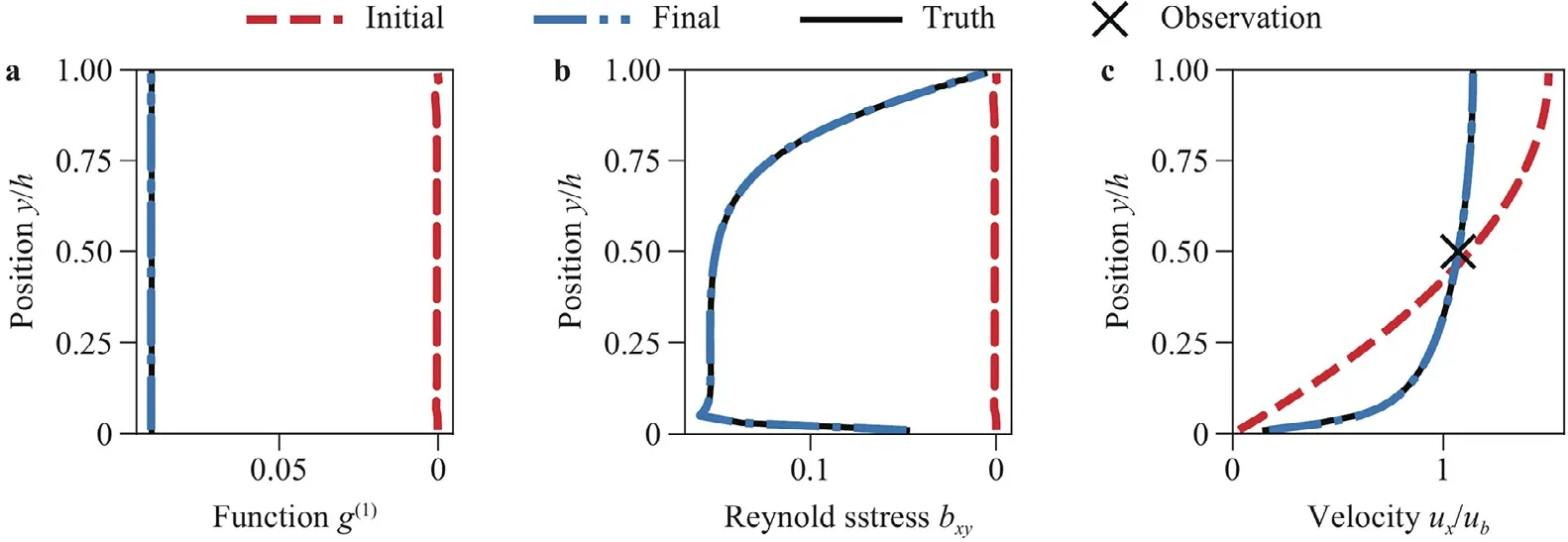
Fig.2.Results of learning a LEVM from a single velocity measurement in a turbulent channel flow: a the learned coefficient function, b the anisotropic Reynolds stress field,and c the velocity.The final (trained) results overlap with the truth and the two are visually indistinguishable.

The viability of the proposed framework is demonstrated by testing on three test cases.The first two cases use synthetic velocity data obtained from a linear and a non-linear closure,respectively,to train the neural network.The use of synthetic data allows us to evaluate the ability of the training framework to learn the true underlying turbulence closure when one exists.In the final test case realistic velocity measurements,obtained from a DNS solution and for which no known true underlying closure exists,are used to learn a linear eddy viscosity model.The trained LEVM is then used to predict similar flows and the predictions are compared to those from a traditional LEVM.

Learning a Synthetic LEVM from Channel Flow

As a first test case we use a synthetic velocity measurement at a single point from the turbulent channel flow to learn the underlying linear model.The flow has a Reynolds number of 10,000 based on bulk velocityuband half channel heighth.The turbulent equations used are thek–ωmodel of Wilcox [28],and the synthetic model corresponds to a constantg(1)=0.09.For the channel flow there is only one independent scalar invariant andT(1)is the only linear tensor function in the basis.We therefore use a neural network with one input and one output which mapsThe network has 1021 trainable parameters and ispre-trainedtothelaminarmodelg(1)=0.The sensitivity of the predicted point velocity to the Reynolds stress is obtained by solving the adjoint equations withJΩequal to the velocity field times a radial basis function (see Appendix B).Figure 2 shows the results of the training.The trained model not only results in the correct velocity field,but the correct underlying model is learned.

Learning a Synthetic NLEVM from Flow Through a Square Duct

As a second test case we use a synthetic full field velocity measurement from flow in a square duct to learn the underlying nonlinear model.The flow has a Reynolds number of 3,500 based on bulk axial velocityuband half duct side lengthh.This flow contains a secondary in-plane flow that is not captured by LEVM [1].For the objective function,JΩis the difference between the measured and predicted fields,with the discrepancy of the in-plane velocity scaled by a factor of 1000 as to have a similar weight to the axial velocity discrepancy.The NLEVM is the Shih quadratic model[29] which,using the basis in Eq.(3),can be written as [27]:

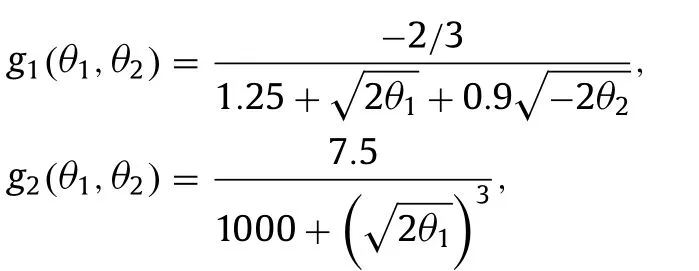
For the flow in a square duct only four combinations of the Reynolds stress components affect the predicted velocity [1]:τxyandτxzin the axial equation andτyzand(τzz−τyy)in the in-plane equation.In this flow the in-plane velocity gradients are orders of magnitude smaller than the gradients of the axial velocityux.For these reasons only two combinations of coefficient functions can be learned [27],g(1)and the combinationg(2)−0.5g(3)+0.5g(4),and there is only one independent scalar invariant withθ1≈−θ2.

The neural network has two inputs and four outputs and was pre-trained to the LEVM withg(1)=−0.09.The turbulent equations used are those from the Shih quadratick–εmodel.Figure 3 shows the learned model which shows improved agreement with the truth.The combinationg(2)−0.5g(3)+0.5g(4)shows good agreement only for the higher range of scalar invariantθ1.This is due to the smaller scalar invariants corresponding to smaller velocity gradients and smaller magnitudes of the tensorsT.The velocity field is therefor expected to be less sensitive to the value of the Reynolds stress in these regions.It was observed that the smaller range of the invariant,where the learned model fails to capture the truth,occurs mostly in the center channel.Figure 4 shows the ability of the learned model to capture the correct velocity,including predicting the in-plane velocities,and the Reynolds stress.The trained model fails to predict the correctτyzin the center channel,but this does not propagate to the predicted velocities.Additionally,it was observed that obtaining significant improvement in the velocity field requires only a few tens of training steps and only requires the coefficients to have roughly the correct order of magnitude.On the other hand obtaining better agreement of the scalar coefficients took 1–2 orders of magnitude more training steps with diminishing returns in velocity improvement.This shows the importance of using synthetic data to evaluate the ability of a training framework to learn the true underlying model when one exists rather than only comparing the quantities of interest.

Learning a LEVM from Realistic Data of Flow Over Periodic Hills

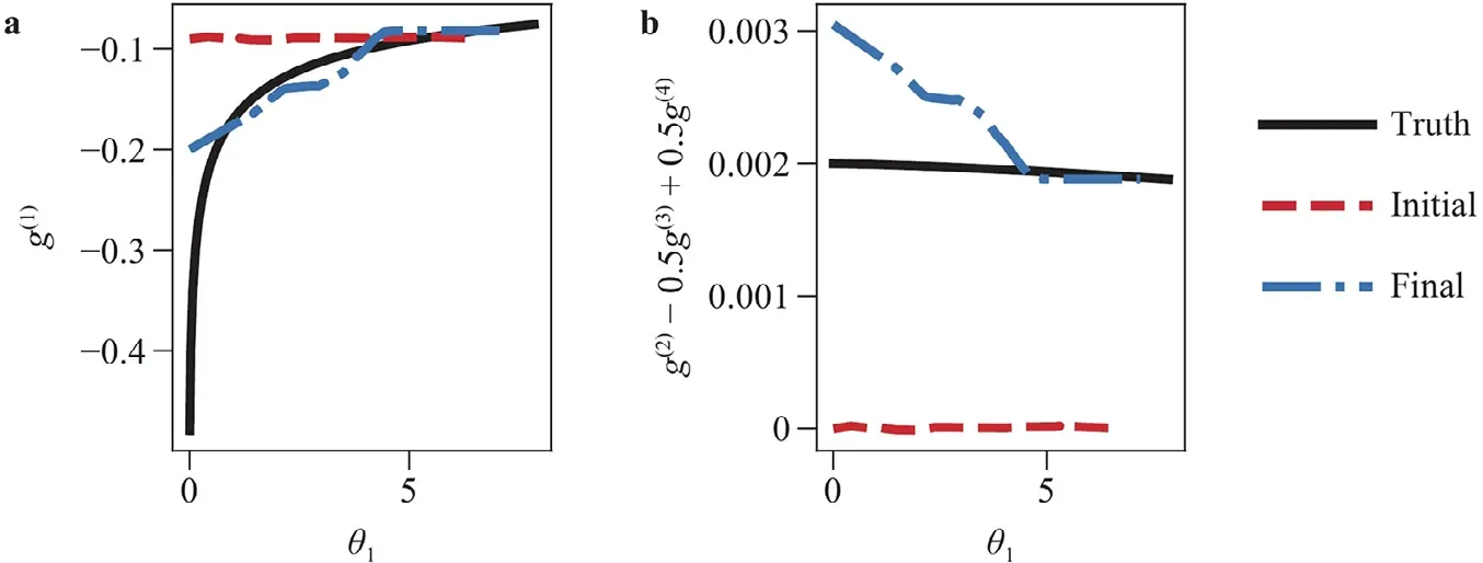
Fig.3.Results of learning a NLEVM,the Shih quadratic model,from full field velocity measurements in flow through a square duct.The results shown are the two combinations of coefficient functions that have an effect on velocity plotted against the scalar invariant θ1≈−θ2.

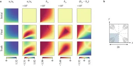
Fig.4.a Velocity and anisotropic Reynolds stress results of learning a NLEVM from full field velocity measurements in flow through a square duct.The uz and bxz fields are the reflection of uy and bxy along the diagonal.b Schematic of flow through a square duct showing the secondary in-plane velocities.The simulation domain (bottom left quadrant) is highlighted.

Fig.5.Velocity results of learning an eddy viscosity model from sparse velocity data of flow over periodic hills.Six different profiles of ux velocity are shown.The training case corresponds to the baseline geometry α=1.

As a final test case,a LEVM is trained using sparse velocity measurements from DNS of flow over periodic hills.The DNS data comes from Xiao et al.[30] who performed DNS of flow over periodic hills of varying slopes.This flow is characterised by a recirculation region on the leeward side of the hill and scaling the hill width (scale factorα) modifies the slope and the characteristics of the recirculation region (e.g.from mild separation forα=1.5 to massive separation forα=0.5).For all flows,the Reynolds number based on hill heighthand bulk velocityubthrough the vertical profile at the hill top isRe=5,600.The training data consists of four point measurements of both velocity components in the flow over periodic hills with the baselineα=1 geometry.The two components of velocity are scaled equally in the objective function.The training data and training results are shown in Fig.5.The neural network in this case has one input and one output and is pre-trained to laminar flow,i.e.g(1)=0.The trained model is a spatially varying LEVMg(1)=g(1)(θ1)that closely predicts the true velocity in most of the flow with the exception of the free shear layer in the leeward side of the hills.

To test the extrapolation performance of the trained LEVM,we use it to predict the flow over the other periodic hill geometries,α∈[0.5,0.8,1.2,1.5],and compare them to results with thek–ωmodelg(1)=−0.09.The results forα=0.5 andα=1.5 are shown in Fig.6.For theα >1.0 cases the trained linear model outperforms thek–ωmodel in the entire flow.For theα <1.0 cases the trained model results in better velocity predictions in some regions,particulary the upper channel,while thek–ωmodel results in better velocities in the lower channel.

Fig.6.Comparison of horizontal velocity ux predictions using the trained eddy viscosity model g(1)=g(1)(θ1) and the k–ω model g(1)=−0.09 on two periodic hills geometries: a α=0.5 and b α=1.5.

In this paper we present a framework to train deep learning turbulence models using quantities derived from velocity and pressure that are readily available for a wide range of flows.The method was first tested using synthetic data obtained from two traditional closure models:the lineark–ωand the Shih quadratick–εmodels.These two cases demonstrate the ability to learn the true underlying turbulence closure from measurement data when one exists.The method was then used to learn a linear eddy viscosity model from synthetic sparse velocity data derived from DNS simulations of flow over periodic hills.The trained model was used to predict flow over periodic hills of different geometries.

This work demonstrates that deep learning turbulence models can be trained from indirect observations when the relevant sensitivities of the RANS equations are available.With the growing interest in differentiable programming for scientific simulations,it is expected that the availability of derivative information will become more commonplace in scientific and engineering computations,making it more seamless to couple scientific computations with novel deep learning methods.Future works include investigating different or multiple types of observation data (e.g.,surface friction,drag and lift coefficients) and parametric studies of locations of observations on the learned model.

Declaration of Competing Interest

The authors declare that they have no known competing financial interests or personal relationships that could have appeared to influence the work reported in this paper.

Acknowledgements

This material is based on research sponsored by the U.S.Air Force under agreement number FA865019-2-2204.The U.S.Government is authorised to reproduce and distribute reprints for Governmental purposes notwithstanding any copyright notation thereon.

Appendix A.Derivation of adjoint equations

The adjoint equations derived here provide the sensitivity of a cost functionJ=J(u,p)with respect to the Reynolds stressτsubject to the constraint thatτ,u,andpmust satisfy the RANS equations.The procedure and notation used here is similar to that in Ref.[24],who derived the adjoint equations for the sensitivity of the Navier–Stokes equations with Darcy term to the scalar porosity field.For detailed derivation of the boundary conditions,which are identical for both cases,the reader is referred to Ref.[24].

The RANS equations can be written asR(u,p,τ)=0 whereand

The minimization of the cost functionJsubject to the RANS constraintR=0 can be formulated as the minimization of the unconstrained Lagrangian function

whereΩis the flow domain andψ=consists of four Lagrange multipliers withreferred to as adjoint velocity and adjoint pressure.The negative of the adjoint pressure is used as the Lagrange multiplier so that in the resulting adjoint equations the adjoint pressure plays an analogous role to that of the physical pressure in the RANS equations.Since the velocity and pressure depend on the Reynolds stress,the total variation ofLis

Here we have ignored the variation of the momentum source termg,which is correct only when the source term is constant,i.e.it does not depend on the other flow variables.If the momentum source term depends on the other flow variables,e.g.to achieve a prescribed bulk velocity as in the test cases used here,ignoring its variation constitutes an approximation.This is similar to the frozen turbulence approximation common in many adjoint-based optimization works [31],where the variations of the turbulence quantities are ignored.Since the constraintR(u,p,τ)is zero everywhere,the Lagrange multipliers can be chosen freely and are chosen such that

to avoid calculating the sensitivities of the other flow variables (u,p) with respect to the Reynolds stress.Equation (A4) is the adjoint condition which leads to the adjoint equations and boundary conditions.Equation (A3) becomes

which leads to an expression for the desired sensitivity∂L/∂τin terms of the adjoint variables.

The variations ofLare obtained as

with the variations of the RANS equationsRas

where the higher order term(δu·∇)δuinδuRwas ignored.Using these results,Eq.(A4) becomes

Integration by parts is used to eliminate the sensitivity of gradients (e.g.∇·δu) from the expression.The results of integration by parts are summarized in Table A1,whereΓ=∂Ωis the boundary of the domainΩ.Integration by parts is done twice on the term with second order derivative ∇2δuwhich leaves a first order derivative in the boundary integral.The termdoes not require integration by parts,but doing so leads to a more convenient adjoint equation that requires only the primal velocity and not its gradient.Finally,the cost functionJis written in terms of integrals over the interior domain and the boundary as

Table A1 Integration by parts written as

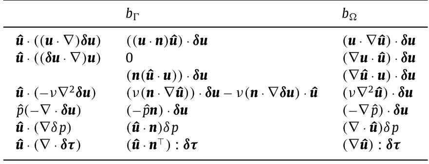
Table A1 Integration by parts written as

and Eq.(A8) can be written as

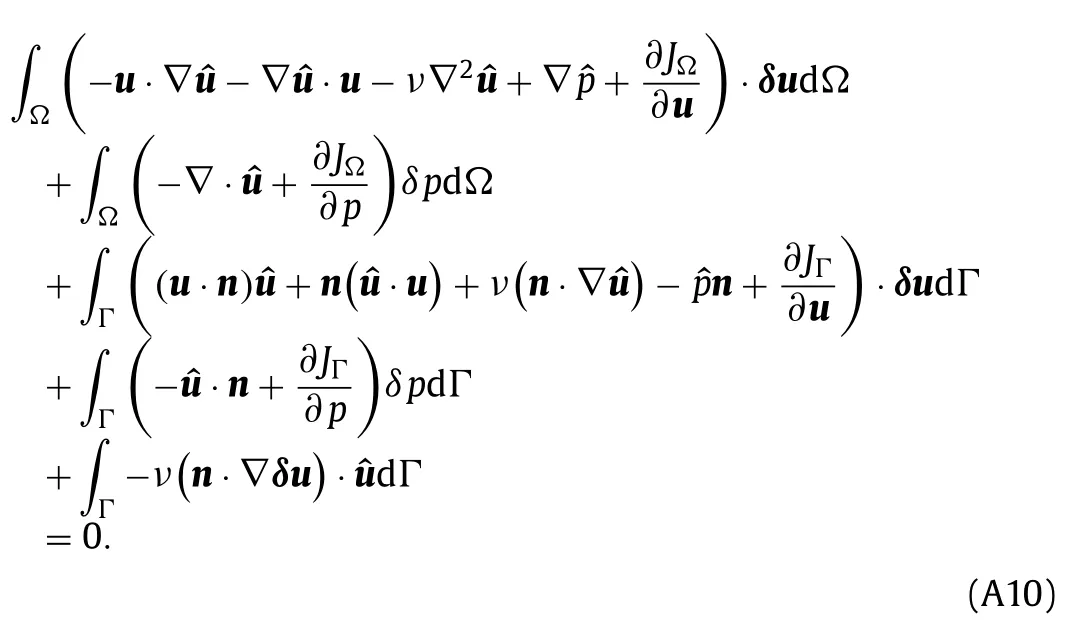
The volume and boundary integrals must vanish separately and the volume integrals will lead to the adjoint equations while the boundary integrals lead to the boundary conditions.

Adjoint equations

The adjoint equations are obtained by requiring the volume integral terms to vanish as

Since Eq.(A11) must hold for any perturbationsδuandδpthat satisfy the RANS equations,the bracketed terms in each of the two integrals must vanish independently.This results in the adjoint equations

a set of linear partial differential equations.

Boundary Conditions

The boundary conditions are obtained from setting the boundary integrals in Eq.(A10) to zero and requiring terms that involveδuandδpto vanish independently as

This can be used to derive the adjoint boundary conditions corresponding to different primal boundary conditions.The resulting adjoint boundary conditions for two typical primal boundary conditions are derived in Othmer [24] and summarized here.The first is a primal boundary with constant velocity and zero pressure gradient,such as a wall or inlet.The corresponding adjoint boundary conditions are

where ∇tis the tangential,in-plane,component of the gradient.Equation (A15a) is used to determine the boundary values of the tangential component of the adjoint velocity.Equation (A15b) then gives a relation between the normal component of the adjoint velocity and the adjoint pressure that can be satisfied by enforcing the resulting adjoint pressure.

Sensitivity

We now derive an expression for the sensitivity of the Laplace function with respect to the Reynolds stress tensor in terms of the adjoint variables.Using the variations in Eqs.(A6) and (A7) and integration by parts (Table A1),Eq.(A5) becomes

Based on Eq.(A16) the sensitivity ofLwith respect to the Reynolds stress at a pointxiin the domain is

and with respect to a pointxiin the boundary it is

Appendix B.Formulation of objective functions

The adjoint method requires the function for which the gradient is sought to be expressible as integrals over the domainΩand boundaryΓ=∂Ωas

This appendix presents how to express the objective function in this manner for some typical experimental measurements.

Full Field or Full Boundary Measurements

First,as a straightforward case,we consider full field or boundary measurements such as full field velocity or pressure distribution along a wall boundary.In these cases the objective function,i.e.the discrepancy between predicted and measured quantities,can be directly expressed in the form in Eqs.(B1).For instance,for full field velocity discrepancy the objective function based on mean squared error is given by

where the superscripts ∗indicates experimental values,and its derivatives are

Similarly,for the pressure distribution along a wall the objective function is given byJΩ=0 andfor points on the wall boundary andJΓ=0 for points on any other boundaries.

Sparse and Integral Measurements

Next,we consider an objective function for the mean squared error discrepancy of more general experimental measurements including sparse measurements such as point velocity measurements or integral quantities such as drag on a solid boundary.The objective function is written as

whered∗is a vector of measurements,Ris the measurement’s covariance matrix that captures the measurement uncertainties,andindicates the L2-norm of a vectorxwith a weight matrixW.The RANS predicted measurements can be written as

with eachJ(i)written in the form in Eq.(B1).The required sensitivity for the objective function in Eq.(B4) is given by

whereithrow of the sensitivity matrixd′(τ)is given by∂J(i)/∂τobtained by solving the adjoint equations with functionJ(i).This requires one adjoint solve for each measurement.For the common situation where the measurements are independent,Ris diagonal with entries corresponding to the variance of each measurementand Eq.(B6) can be written as

where the discrepancy for each measurement is weighted by the measurement’s variance.Alternatively,for the purpose of learning a turbulence model one might want to weight different types of measurements differently,e.g.to manually give more weight to regions of rapid change such as in boundary and shear layers or use a more formal importance sampling approach.The weighting in Eq.(B7) becomesand the weight matrix in the norm in Eq.(B4) becomeswhere the vector of weightsλ=andDλis the diagonal matrix with entriesλ.

We now provide two concrete examples of expressing measurement discrepancies in the form of Eqs.(B4) and (B5).First,for a single point measurement ofux,

where the mask fieldMis the Dirac delta functionδifor the measurement location.For the discretized problem the mask can be approximated using a radial functionrcentered at the measurement location,and normalized such that the integral of the mask field is one.As a second example,for the drag on a wall boundary,

wherexDis the unit vector in the direction of drag and the mask is one for points on the wall boundary and zero for points on any other boundaries.