Short Matlab programs for time and frequency response of MDOF system by mode superposition methods
2021-09-07WANGBopingZHANGJunru
WANGBo-ping,ZHANGJun-ru
(1.Department of Mechanical and Aerospace Engineering,University of Texas at Arlington,Arlington 76019,USA;2.State Key Laboratory of Structural Analysis for Industrial Equipment,Dalian University of Technology,Dalian 116024,China)
Abstract: Matlab programs for vibration responses analysis are presented in this paper.These programs can be used for time and frequency domain solution of linear discrete systems described by mass,stiffness matrices M and K and general viscous damping matrix.Mode superposition formulations are used to compute the solutions.For undamped systems,the user can select either numerical or symbolic solutions(in terms of time or frequency).Numerical solutions are computed for damped system via superposition of complex modes.Mode superposition methods are summarized and implemented in several short Matlab programs.Various cases of a three degrees-of-freedom system and a cantilever beam model are used to illustrate the application of the programs.These programs can also be used in industrial application by post-processing mass and stiffness matrixes generated by commercial finite element package to produce time or frequency response of interest.
Key words: Matlab programs;time and frequency response;multi-degree of freedom system(MDOF);mode superposition methods
1 Introduction
Vibration (or structural dynamics) analysis is an important field in engineering.To improve product quality and service life,reducing vibration responses plays an important role in the design of buildings,bridges,ground vehicles,ships and aerospace structures.A thorough understanding of vibration theory and the associated computation is the foundation to achieve vibration reduction in engineering design.The objective of this paper is to present Matlab implementation of well-known analytical mode superposition solutions for time and frequency domain analysis of linear discrete systems.Both undamped and generally viscously damped system are considered.
Nowadays,due to its modern computing and graphical visualization capabilities,Matlab has been extensively taught in Universities and applied in industry.The Matlab programs presented in this paper can be used to validate results computed by other methods.In 2005,Bingen Yang published a textbook[1]with interactive Matlab computing in solid and structural mechanics,including vibration analysis and structural dynamics.Yang’s book provided tools for free and forced responses analysis of MDOF systems.But he considers only undamped or proportionally damped system.He provided formulations for generally damped system but did not provide tools for implementation.For frequency response analysis,Yang provided tools for general system by direct solution (i.e.inverse (K+iωC-ω2M) for each frequency).The tools provided in this paper apply the mode superposition methods(or modal analysis)to find solution for both time and frequency domain solutions(complex modes are used for generally damped system in our tools).It can also be used for parametric study to understand the effect of parameters.These programs can be also used in design optimization.
The following is the organization of the paper. In Section 2,the vibration problem to be solved is described.Eigenvalue problems for undamped and damped systems are also discussed in this section.Mode superposition methods for computing time domain responses are presented in Section 3 and 4.Since these solutions are well known and can be found in many textbooks[2-10],summary of the solution procedures is presented without derivation.Section 5 presents frequency response solutions under mode superposition.Note that both undamped and damped system are considered in the above formulation.For damped system,complex modes are used in mode superposition.Section 6 describes Matlab implementation of the formulations of Section 3 and 5.Various solutions of a 3-dof Example and a cantilever beam model are presented in Section 7 to illustrate the application of various programs.A brief conclusion is given in Section 8.Listings of Matlab programs are presented in the Appendix.
2 Equation of Motion and eigenvalue problems
Equation (1) is the equation of motion (EOM) for the MDOF system studied in this paper,
(1)
whereM,C,Kare mass,damping and stiffness matrices respectively.uis the displacement vector and dots represents time derivatives.f(t) is the forcing function vector and its form depends on the solution type,time and frequency domain,described in the next two sections.
For a generally damped system,the EOM is usually cast into the following first order or state space form,

(2)
where
(3)
(4)
Note that
(5)
and
(6,7)
2.1 Eigenvalue problem for undamped free vibration
For undamped,free vibration leads to the following generalized eigenvalue problem,

(8)

Many numerical methods are available to solve this problem.In this paper,we will solve this problemby using Matlab function eig.This is achieved by the following command,
[Φ,λ]=eig(K,M)
(9)
Note that modesrands(r≠s)areM-orthogonal andK-orthogonal to each other,that is,

(10a,10b)
2.2 Eigenvalue problem for damped free vibration
For free vibration Eq.(2) leads to the following eigenvalue problem,
Aψ=λψ
(11)
Since matrixA is not symmetric,we also need to solve the following Left Eigenvalue problem,
ATψL=λψL
(12)
Note that the above eigenvalue problems have same eigenvalue solutions but the corresponding eigenvectors are different.
For anN-dof system,the matrix A in Eq.(3) is of order 2N.The 2Ncomplex eigenvalues areNconjugate pairs.Thus,letλ1,λ2,…,λ2 N - 1,λ2 Nbe the 2Neigenvalues andΨ1,Ψ2,…,Ψ2 N - 1,Ψ2 Nbe the corresponding eigenvectors,then,
(13,14)
where the superstar indicated complex conjugate.
Furthermore,letΨL 1,ΨL 2,…,ΨL 2 N - 1,ΨL 2 Nbe the left eigenvectors,then the following are the bi-orthogonal properties of the eigenvectors,that is,forr≠s,
(15a,15b)
3 Time domain solutions of undamped vibration
For time domain solutions,we assume the forcing function is composed of constants,sine and cosine terms.That is,
f(t)=P0+Pssin(Ωst)+Pccos(Ωct)
(16)
Additionally,the following Initial Conditions(IC) are required for time domain solutions,
u(0)=u0,v(0)=v0
(17)
Using mode superposition method,the time response in matrix form can be calculatedby using the well-known following equation,

(18a,18b)
where ther-th modal coordinatesqr(t) are computed by using the following analytical solutions of the following equation,
(19)


(20a,20b)
The modal initial conditions are,
(21a,21b)
Use the above data,Eq.(19) can be solved.We will find solutions due to initial conditions and different terms of forcing functions separately.There are summarized below.
3.1 Response to initial condition
For response due to initial condition only,f(t)=0.HenceGFr(t)=0.Thus,use SDOF formula,
(22)
3.2 Response to step input
For step input with zero initial conditions,the EOM forqr(t) is,
(23)
whereP0is the step force.Thus,
(24)
3.3 Response to sinusoidal input
For non-resonant sine inputPssin(Ωst) with zero initial condition the EOM forqr(t) is,
(25)
whereΩsis the forcing frequency in the sine terms,Ωs≠ωr.The solution is,
(26)
3.4 Response to cosine input
For non-resonant cosine inputPccos(Ωct),with zero initial condition the EOM forqr(t) is,
(27)
whereΩcis the forcing frequency in the cosine terms,Ωc≠ωr.The solution is,
(28)
The total modal response to initial conditions and loading is the summation of the above responses.
4 Time domain solutions of damped vibration
For damped systems,the time domain response of states can be calculatedby using the following equation,
(29)
Or in matrix form
x(t)=Ψq(t)
(30)
where modal states are the solution of the following first order ordinary differential equation,
(31)

(32)
and initial conditions
(33)
Specifically,solutions to IC and different force terms are summarized below.
4.1 Response to initial condition
For response due to IC only,GFr(t) equals zero.The solution of Eq.(31) is,
qr(t)=qr(0)eλrt
(34)
4.2 Response to step input
Modal response due to constant step forceP0and zero initial condition is,
(35)
4.3 Response to Sinusoidal Input
Modal response due tosinusoidal inputPssin(Ωst) with zero IC’s is,
(36)
4.4 Response to Cosine Input
Modal response due tocosine inputPccos(Ωct) with zero IC’s is,
(37)
5 Frequency Domain Solutions of
undamped and damped vibration
The forcing function for frequency response is,
f(t)=Pei Ω t
(38)
The corresponding solution is,
u(t)=U(Ω)ei Ω t
(39)
For undamped system,the solution by using mode superposition method is,
U=ΦQ
(40)
where
(41)

(42)
For damped system,the solution by using mode superposition method is
(43)
(44)
6 Implementation
The formulations summarized in the previous two sections are implemented in the two Matlab programs (functions) described below.These programs areModal_Time_Funfor time domain analysis andModal_Freq_Funfor frequency domain analysis.Additionally,the time domain function is applied twice in programModal_Pulse_Funto solve for pulse responses.The following are commands to use the three programs,
[U,V]=Modal_Time_Fun(K,M,C,u 0,v 0,P 0,Pc,Wc,Ps,Ws,time);
[U,V]=Modal_Freq_Fun(K,M,C,PW,WW);
[UF,UR,tF,tR]=Modal_Pulse_Fun(K,M,C,u 0,v 0,P 0,Pc,Wc,Ps,Ws,t 1,T 0);
The input data to these functions are summarized in Table 1.The following is a brief description of output computed by these programs.
For time domain solutions the outputs are U=displacement,V=velocity responses.For undamped system,U,V=symbolic form of solutions.This is achieved by specifying data for time point as 0 (i.e.,time=0).If a list of time points is provided in the inputs,U,V=numerical solutions.
For frequency domain solutions the outputsare U,V=amplitude displacement and velocity responses.For undamped system,U,V=symbolic form of solutions.If data for frequency points is 0 (i.e.,WALL=0),otherwise,if a list of time points is provided in the inputs,U,V=numerical solutions.

Tab.1 Input for solution function
For pulse responses solutions the outputs are: If time=0,UF,UR=symbolic form of forced responses and residual vibration respectively (undamped system only).Forced responses are the responses when the applied load is active.After the applied loading ceases to apply,the motion is referred to residual vibration.These vibration are induced by non-zero displacements and velocities at the end of the forcing period.Otherwise,UF,UR=numerical solution of forced responses and residual vibration respectively and tF,tR=corresponding time points for forced response and residual vibration.
It should be noted that in the mode superposition formulation,three loops(do -loop in FORTRAN of for-loop in Matlab) are required to compute the responses at each degree-of-freedom(dof).One loop for dof-number,one for mode number and one for time (or frequency) points.In the codes presented in the Appendix,only one loop is used to compute responses of modal coordinates.Mode-superposition to obtain physical responses are implemented as matrix-product without addition for-loop.
7 NumericalExamples
7.1 3-dofs dampedspring-mass model
Consider the 3-dofs system shown in Fig.1,

Fig.1 A 3-dofs damped spring-mass model
WithM1=4,M2=2,M3=4 kg,K1=100,K2=600,K3=800 N/m,C1=10,C3=10 N·s/m (for undamped case,C1=C3=0).Note that this is non-proportional damping.The system matrices are,
(45a)

(45b)
(45c)
A rectangular pulse input is applied,
T0=1.5s
(46)
Matlab programModal_Pulse_Funis used to solve for the time response for both undamped and damped systems.The solutions can be divided into two parts:forced response whent≤T0and residual vibration whent>T0.For undamped system,the forced response is,
u1(t)=0.005-0.005383cos(8.546t)+
0.0003828cos(32.05t)
u2(t)=0.01333-0.01173cos(8.546t)-
0.0016cos(32.05t)
u3(t)=0.01333-0.01435cos(8.546t)+
0.001021cos(32.05t)
(47)
The residual vibration is,
u1(t)=0.0001704cos(8.546t-12.82)+
0.001344sin(8.546t-12.82)-
0.0006068cos(32.05t-48.07)+
0.0003104sin(32.05t-48.07)
u2(t)=0.0003715cos(8.546t-12.82)+
0.002929sin(8.546t-12.82)+
0.002536cos(32.05t-48.07)-
0.001297sin(32.05-48.07)
u3(t)=0.0004545cos(8.546t-12.82)+
0.003583sin(8.546t-12.82)-
0.001618cos(32.05*t-48.07)+
0.0008277sin(32.05t-48.07)
(48)
The pulse responses are also computed numerically for both damped and undmped.The results are plotted in Fig.2.
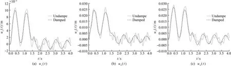
Fig.2 Pulse responses for both the damped and undamped
For frequency response,the input force is,
(0≤Ω≤40 rad/s)(49)
The undamped symbolic solutions are,
(50)

Fig.3 Frequency responses for both the damped and undamped
7.2 Beam model
Consider the cantilever beam model of Fig.4 with a force applied at the tip.

Fig.4 Beam model


Fig.5 Beam elements
For time domain response,the input force is given,f(t)=Pssin(20t)
(51)
By using the Matlab implementation of the method in this paper,the time domain responseuyof tip node is plotted below and we compared it to the results of ANSYS.The time domain response curves of ANSYS or matlab are coincided which proves the effectiveness of the method used in this paper.ANSYS or matlab code use the same classic Euler-Bernoulli beam element.

Fig.6 Time domain responses by using Matlab
For frequency response,the input force is given,
f(t)=Pei Ω t(0≤Ω≤2000 rad/s)
(52)
Numerical frequency responseuyof tip node are computed for undamped cases.The frequency response is plotted in Fig.7.
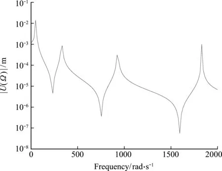
Fig.7 Frequency responses by using the direct method
8 Conclusions
The programs presented in this paper can be used to find time and frequency responses of linear systems.For time domain problem,responses to initial conditions and combination of constant (step) and sinusoidal forces can be calculated.Both damped and undamped systems are considered in time and frequencydomain solution.Numerical solutions are computed at the user specified time or frequency points.For undamped system,symbolic outputs in term of time or frequency parameter are available.The source listing of the main programs is included in the paper.These programs can be extended to solve problems not covered by the two main programs.Specifically,the programModal_Pulse_Funis a direct extension of the time domain program to solve for pulse responses of MDOF systems.
Using these programs,the user can perform parametric study to gain more understanding of the vibration being investigated.This can be achieved by simply changing input data without the need to write a program for each case.Additionally,these program can be extended easily to handle system with rigid modes,base excitation and other applications.Finally,it should be noted that these programs can also be applied to solve SDOF (single-degree-of-freedom) vibration problems.
Appendix
Listing of Modal_Time_Fun:

Listing of Modal_ Pulse _Fun:
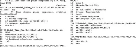
Listing of Modal_ Freq _Fun:

