A time -variant reliability analysis method based on interval process model

LIJin-wu,LIJin-yang,JIANGChao,NIBing-yu,YANGGang

(College of Mechanical and Vehicle Engineering,State Key Laboratory of Advanced Design and Manufacturing for Vehicle Body,Hunan University,Changsha 410082,China)

Abstract: In this paper,a time-variant reliability analysis method based on the interval process model is proposed to deal with problems involving interval variables and interval processes.A reliability index based on the extreme response is first defined to measure the reliability of a structure under uncertainties modeled by interval variables and interval processes.Then a double -loop optimization is developed to calculate the reliability index.In the inner loop,the extreme response with respect to time is calculated using the efficient global optimization method.In the outer loop,an optimization with respect to all input interval variables,including the original ones and those obtained after the series expansion of the input interval processes,is performed to search for the upper and lower bounds of the extreme response.Two examples are used to demonstrate the effectiveness of the proposed method.

Key words: time -variant reliability analysis;interval process model;interval K-L expansion;extreme response

1 Introduction

In practical engineering,a structure usually suffers from material degradation and component wear,and may be subjected to time-variant uncertain loads.As a result,the structure’s performances such as displacement exhibit time -variant characteristics and hence the time-variant reliability analysis instead of the conventional static reliability analysis should be considered.So far,a series of time-variant reliability analysis methods have been developed to evaluate the reliability index or failure probability,including outcrossing rate method[1,2],extreme value method[3,4],sampling-based method[5,6],surrogate model based method[7],etc.Among these methods,the outcrossing rate method based on Rice’s formula[8,9]is the most widely investigated and applied in the field of the time-variant reliability analysis with the assumptions that outcrossings are independent mutually and their occurrence follows a Poisson distribution.Nevertheless,the low computational accuracy of the outcrossing method may be encountered in some complex problems due to these assumptions[10].Therefore,the joint outcrossing rate method[11,12]is developed to improve the computational accuracy by relaxing the independence assumption.In the extreme value method,the extreme value of a response function over a specific lifetime is extracted and the reliability analysis is conducted based on the traditional time-invariant method[3,4].In recent years,many newly developed methods are reported in the time-variant reliability analysis community,such as probability density evolution method[13-15],envelope function method[16].

The existing time -variant reliability analysis methods are generally developed based on the probabilistic models[17-19]in which a vast amount of sample information is generally needed for the construction of precise probability distribution of static parameters and time-variant parameters at arbitrary time point.However,due to the limitations in test cost and conditions,it is often difficult to obtain sufficient sample information for the construction of the precise probability distribution in practical engineering.In that case,non-probabilistic models seem to be more applicable than the probabilistic models.

In this paper,the static and the time-variant parameters are modeled by interval variables and interval processes,respectively.Then a corresponding reliability index is proposed to measure the structural reliability considering the input interval variables and processes.Finally,a double -loop optimization is developed to calculate the reliability index.In the inner loop,the extreme response with respect to time is calculated using the efficient global optimization (EGO) method.In the outer loop,an optimization with respect to all input interval variables,including the original ones and those obtained after the series expansion of the input interval processes,is performed to search for the upper and lower bounds of the extreme response.The remainder of the paper is organized as follows: A brief review to the interval process model is given in Section 2.A reliability index and a double-loop optimization method to calculate the index are given in Section 3.Section 4 gives two examples followed by conclusions in Section 5.

2 Fundamentals of interval process theory[20,21]

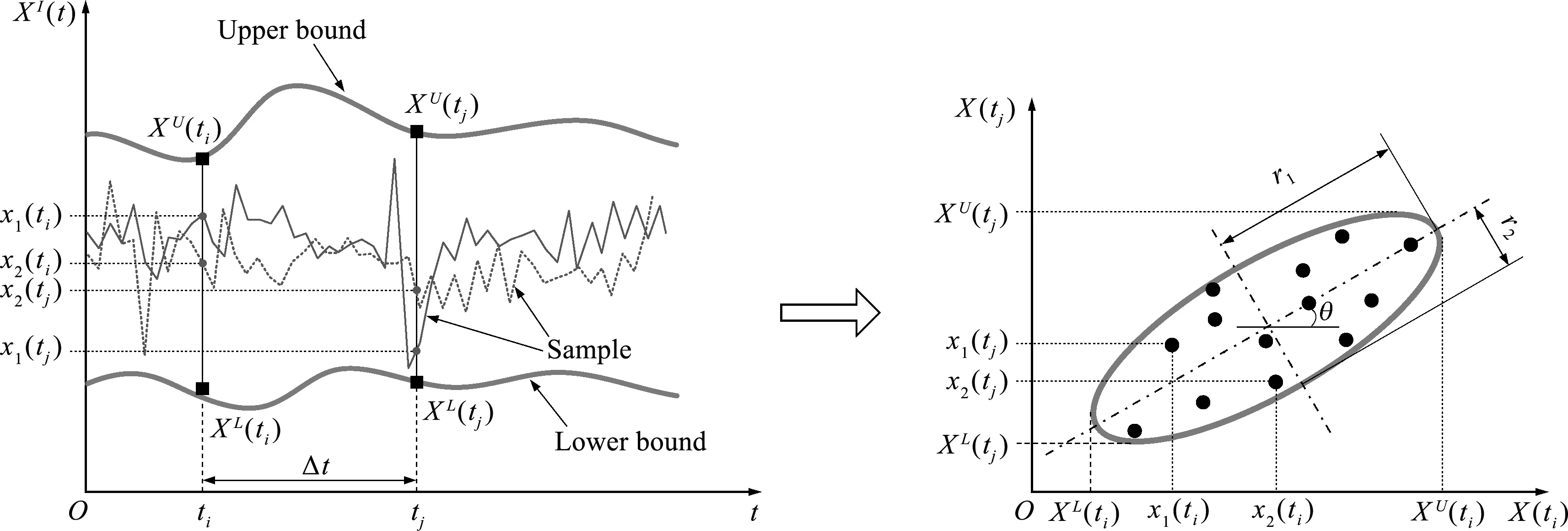
As shown in Fig.1,the interval process model[21]proposed by the authors employs a bounded and closed interval for the quantification of the parametric uncertainty at arbitrary time point,and a specific auto-correlation coefficient function is defined for description of the correlation between the interval variables at arbitrary two different time points.

Fig.1 Interval process model[21]

Definition1.A time -variant uncertain parameter {X(t),t∈T } is an interval process if for an arbitrary timeti∈T (i=1,2,…),the possible values ofX(ti) can be represented by an intervalXI(ti)=[XL(ti),XU(ti)],where T is a parameter set oft.

Definition2.For an interval processXI(t),its middle point functionMXI(t),the radius functionRXI(t) and the variance functionDXI(t) are defined as:

Xm(t)=M[XI(t)]=[XL(t)+XU(t)]/2

(1)

RXI(t)=Xr(t)=[XU(t)-XL(t)]/2

(2)

DXI(t)=D[XI(t)]={[XU(t)-XL(t)]/2}2

(3)

whereXU(t) andXL(t) are the upper bound function and the lower bound function ofXI(t),respectively.

Definition3.For an interval processXI(t),the auto-covariance function of interval variablesXI(ti) andXI(tj) at any two time pointstiandtjis defined as:

(4)

whereθis the relevant angle,r1andr2are the half lengths of the major axis and the minor axis of the ellipse,and they can be obtained based on the samples ofXI(t),as shown in Fig.2.More details on the procedure to compute the auto-covariance function can be referred to our previous works[20-22].

Fig.2 Calculation of the auto -covariance function of an interval process[21]

Definition4.For an interval processXI(t),the auto-correlation coefficient function of interval variablesXI(ti) andXI(tj) at any two time pointstiandtjis defined as:

(5)

Definition5.The cross-covariance function and the cross-correlation coefficient function of interval processesXI(t) andYI(t) are defined as:

(6)

(7)

whereθis the relevant angle,r1andr2are the lengths of the major axis and the minor axis of the ellipse,and they can be obtained based on the samples ofXI(t) andYI(t).

Definition6.If the middle point functionMXI(t) and the radius functionRXI(t) of an interval processXI(t) are both constants and its auto-covariance function is only related to the time intervalτ=|ti-tj| rather than the time pointstiandtj,namely:

MXI(t)=mXI,RXI(t)=rXI

(8,9)

CovXIXI(ti,tj)=CovXIXI(0,τ)=CovXIXI(τ)

(10)

wheremXIandrXIare both constants,CovXIXI(τ) is a function ofτ,then the interval processXI(t) is called stationary interval process.

3 Proposed time-variant reliability analysis method

In this section,the interval process model is used to describe the parametric uncertainties of the time-variant parameters,and a time-variant reliability analysis method is developed,which can reduce the dependence on a large number of samples to a great extent.

3.1 Time -variant reliability modeling under interval processes

Consider a structure with the performance function as follows:

G(t)=g(YI,XI(t),t)

(11)

(12)

Without loss of generality,it is assumed that only one interval processXI(t) is involved in the performance function.By using the truncated interval K-L expansion,the interval process can be represented by the combination of a series of uncorrelated standard interval variables and deterministic functions of time[24]:

(13)

Substituting Eq.(13) into Eq.(11) yields:

(14)

whereζj(j=1,2,…,N) are standard interval variables and form an interval variable vectorζ=[ζ1,ζ2,…,ζN] whose joint uncertainty domain is Ωζ={ζ|ζTζ≤1}.We rewrite Eq.(14) as follows:

G(t)=h(Y,ζ,t)

(15)

whereh(·) can be obtained through a simple transformation ofg(·).LetZ=[YT,ζT]T,and its joint uncertainty domain can be represented as:

(16)

Thus Eq.(15) can be rewritten as:

G(t)=h(Z,t)

(17)

It should be noted thatG(t) is an interval variable at arbitrary time instant sinceZis an interval variable vector.

For a given design lifetimeT,the structure is safe if the extreme response of the performance function is greater than 0 over the whole design lifetime,namely:

(18)

(19)

According to Eqs.(18～19),the event that the structure is safe over the whole design lifetime means that the extreme responseHTis greater than 0.Hence,the time-variant reliability index over the design lifetime is equal to the time-invariant reliability index for a structure whose performance function is the extreme responseHT.

So far,a variety of non-probabilistic reliability analysis models and corresponding algorithms[25-29]have been developed for time-invariant problems.Although these models and algorithms can deal with the non-probabilistic reliability analysis in a certain aspect,this paper gives a new effective reliability index to measure the safe degree of the structure with performance functionHT.

In this paper,the proposed reliability index is defined as:

(20)

(21)

and

(22)

After obtaining the lower and upper bounds for the performance functionHT,the non-probabilistic reliability index can be acquired based on Eq.(20).

3.2 Solution procedure

It can be known from Section 3.1 that the time-variant reliability index over the given design lifetime is equal to the reliability index of a structure with the performance functionHT.To calculate the reliability index,the lower and upper bounds of the performance functionHTwithin the joint uncertainty domain ΩZshould be obtained in advance.The detailed calculation procedure of the non-probabilistic reliability index is summarized as follows:

(1) Give the design lifetimeTfor a structure and the joint uncertainty domain of the interval variable vectorYIand the characteristic parameters of the interval process vectorXI(t).

It should be noted that solving Eq.(21) or Eq.(22) is a double-loop optimization problem in Step (3) in the calculation procedure.The objective of the inner loop optimization is to search the minimum value ofh(Z,t) over the design lifetime with a specific realization of the interval variable vectorZ.The objective of the outer loop optimization is to find the lower bound or upper bound of the performance functionHT.For these two kinds of optimization problems,all of the gradient algorithm[30],intelligent algorithm[31]and EGO method[32]can be used to obtain the optimum solution.In this paper,EGO method is used in both inner loop optimization and outer loop optimization.

4 Numerical examples and discussions

To verify the effectiveness of the proposed time-variant reliability analysis method,a numerical example and a practical engineering case are investigated in this section.

4.1 A numerical example

Consider a numerical example whose performance function is presented as:

g(t)=X(t)

(23)

(1) Effects of the correlation length

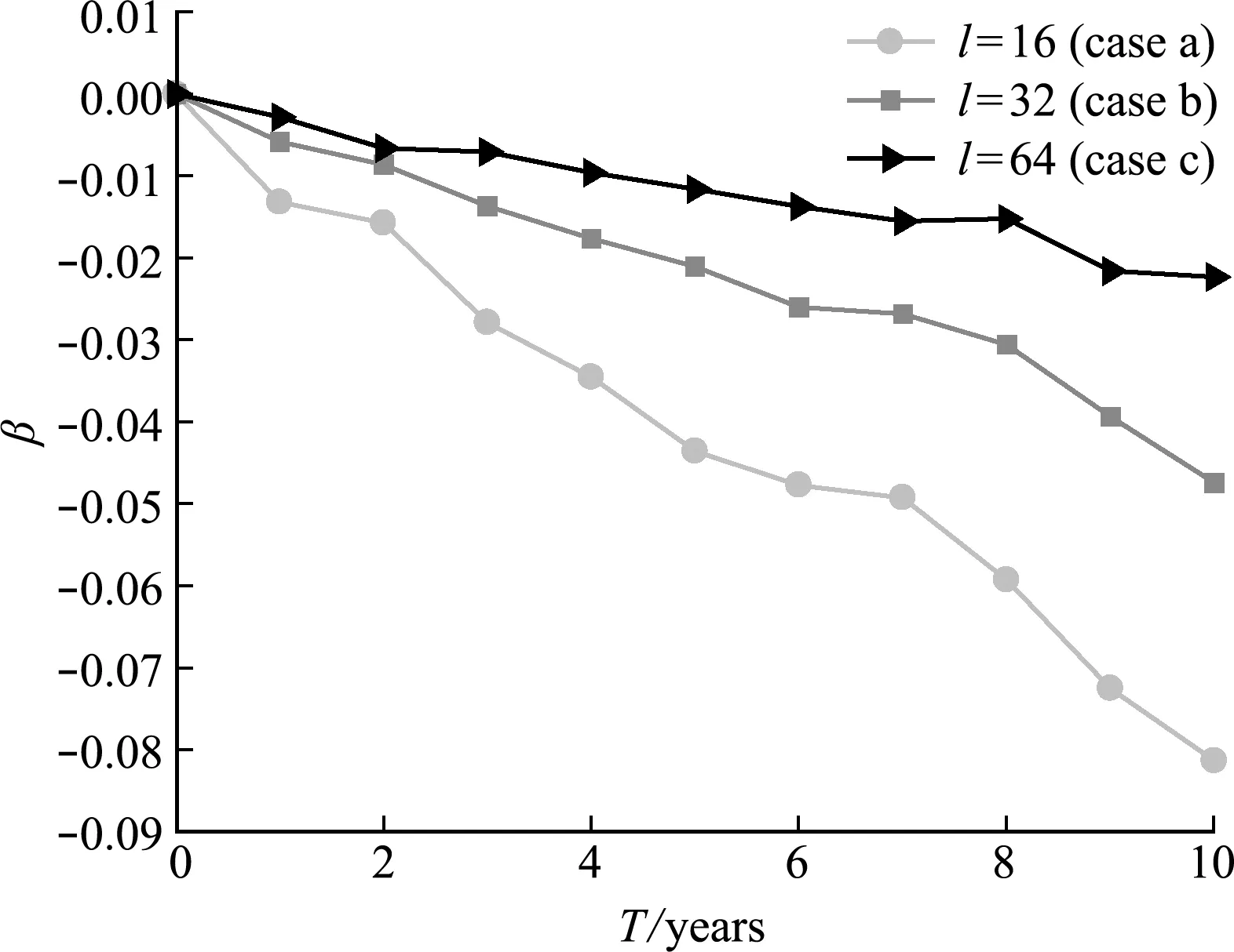
Let the middle point function and the radius function ofXI(t) beXm(t)=0 andXr(t)=1,respectively.Consider three cases for the correlation length:l=16 (case a),l=32 (case b) andl=64 (case c).By using the proposed method,the time-variant reliability indices over various design lifetimes can be calculated as listed in Tab.1,and the corresponding curves are depicted in Fig.3.Firstly,for all of these three cases,the reliability index decreases with the increment of the design lifetime as shown in Fig.3.Secondly,the reliability index increases with the increment of the correlation lengthlfor a same design lifetime.It is because that the increase of the correlation lengthlcauses the decrease of the fluctuation degree of the interval process,which will lead to the increase of the reliability.Thirdly,the reliability indices for all three cases of the correlation lengths are 0 at the initial stage,which indicates that there is no effect of the correlation length on the reliability index of the structure at the initial stage.Finally,the minimum reliability index among these three cases when the design lifetime is 10 years is -0.0814 which occurs when the correlation lengthl=16,indicating that the smaller the correlation length is,the faster the reliability decreases.

Tab.1 Reliability indices for the numerical example over time under different correlation length

Fig.3 Curves of the reliability indices for the numerical example over time under different correlation length

(2) Effects of the middle point function

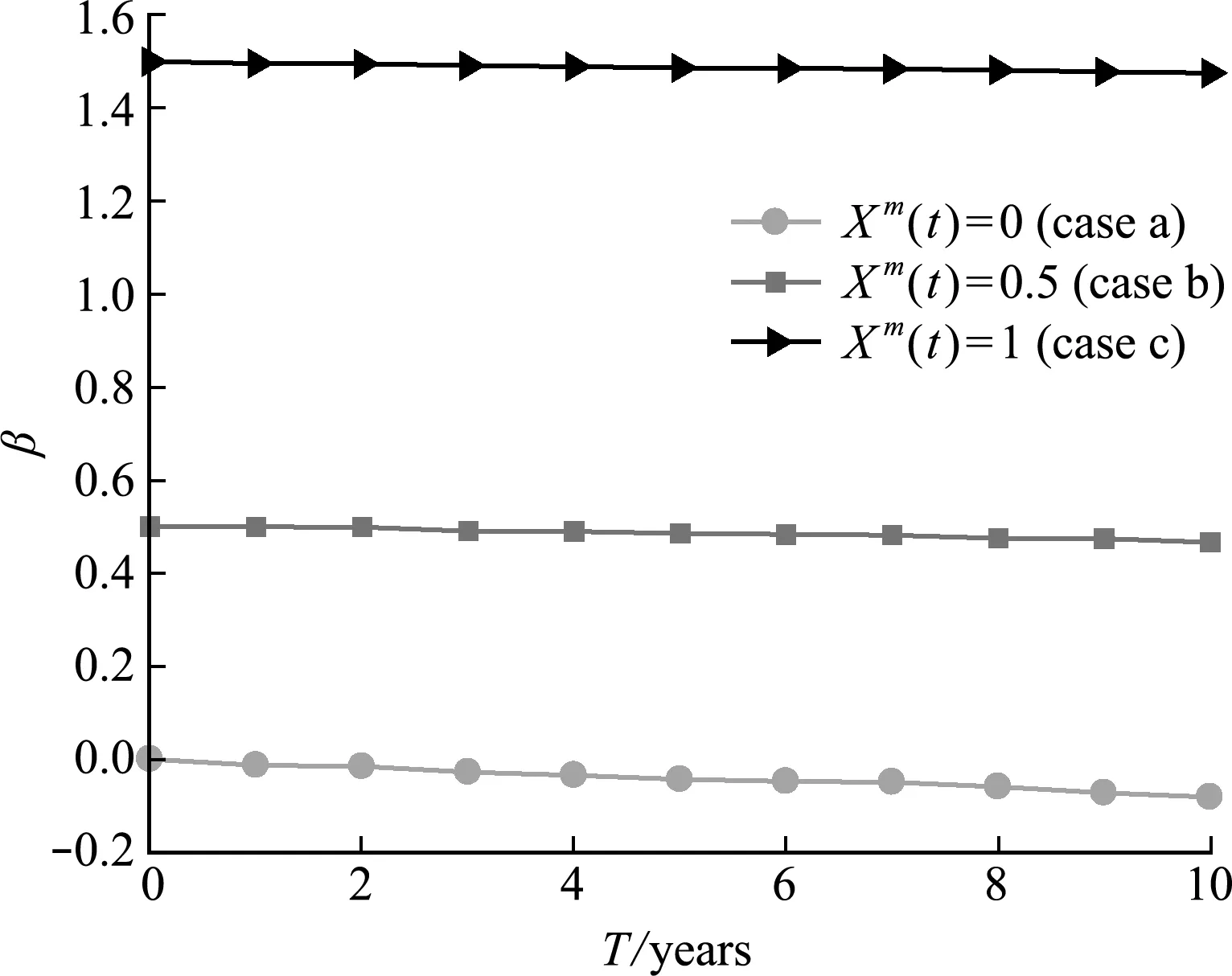
The correlation length in the auto-correlation coefficient function and the radius function of the interval process are treated asl=16 andXr(t)=1,respectively.Consider the following different three cases for the middle point functions:Xm(t)=0 (case a),Xm(t)=0.5 (case b) andXm(t)=1 (case c).By using the proposed method,the time-dependent reliability analysis results can be calculated as listed in Tab.2,and the corresponding curves are depicted as Fig.4.To begin with,for a same design lifetime,the greater value of the middle point function is,the greater reliability index is.For instance,when the design lifetime is 5 years,the reliability indices for these three cases of the middle point function are -0.0436,0.4853 and 1.4866,respectively.In addition,the reliability indices for case c are always not smaller than 1 while this phenomenon does not exist for cases a and b.The reason why the reliability indices for case c are always not smaller than 1 is that the lower bound of the interval process is 0 for case c,which means that all the possible values are not smaller than 0 and the structure is absolutely reliable.

Tab.2 Reliability indices over time under different middle point functions

Fig.4 Curves of the reliability indices over time under different radius functions

4.2 A printed circuit board (PCB) module

The PCB,an important part of the electronic equipment,is widely used in the industry field and its performance has a significant impact on the whole performance of the electronic equipment[33].The time-variant reliability analysis of the PCB module provides a valuable reference to the improvement of the whole performance of the electronic equipment.Fig.5 presents the PCB module of a high-definition camera and its finite element model.The sensor collects signal from the light irradiating on its surface for image formation,and the decrease in the ability of image formation occurs when the thermal deformation of the PCB module is quite large,so the degree of thermal deformation of the PCB module has a significant effect on the property of the high-definition camera.The heat that causes the thermal deformation of the sensor is mainly from chip 1 and chip 2.The outline dimensions of PCB are 68 mm×54 mm×1.2 mm,and the material properties of the module are listed in Tab.3.With the maximum normal deformation in the permission of the sensorD0=0.3 mm and the actual maximum deformationD,the performance function is given by:

Fig.5 A PCB module and its finite element model[33]

Tab.3 Material parameters for the PCB module

g(t)=D0-D(P1(t),P2)

(24)

By using the finite element method,the model of the PCB module is constructed with 22929 hexahedral elements.The finite element model is used for analysis after 65 samples were obtained by Latin hypercube sampling method,and the second-order response surface of the deformationDis then constructed on that basis as follows:

0.0292P1(t)P2+0.225

(25)

Fig.6 Curves of the reliability indices for the PCB module over time under different radius functions

5 Conclusions

This paper proposes a new time-variant reliability analysis method based on the interval process model,providing an effective way for dynamic safety evaluation under insufficient samples.In the proposed method,the time-variant uncertainties are modeled using the interval process model,which reduces the dependence on a large number of samples.The results of the numerical examples indicate that the reliability index decreases with the increase of the design lifetime when the time-variant parameters or dynamic loads are described by the interval process model.Furthermore,there are profound effects of the characteristic parameters of an interval process on the time-variant reliability index.Therefore,it is necessary to consider the effects of a variety of time-variant uncertain factors on the structure in its initial design stage.As a new time-variant reliability analysis method,the proposed method is expected to extend to other fields,such as system time-variant reliability analysis and reliability optimization design.