Physics-informed deep learning for digital materials

Zhizhou Zhang,Grace X Gu

Department of Mechanical Engineering, University of California, Berkeley, CA 94720, USA

Keywords: Physics-informed neural networks Machine learning Finite element analysis Digital materials Computational mechanics

ABSTRACT In this work,a physics-informed neural network (PINN) designed specifically for analyzing digital mate-rials is introduced.This proposed machine learning (ML) model can be trained free of ground truth data by adopting the minimum energy criteria as its loss function.Results show that our energy-based PINN reaches similar accuracy as supervised ML models.Adding a hinge loss on the Jacobian can constrain the model to avoid erroneous deformation gradient caused by the nonlinear logarithmic strain.Lastly,we discuss how the strain energy of each material element at each numerical integration point can be calculated parallelly on a GPU.The algorithm is tested on different mesh densities to evaluate its com-putational efficiency which scales linearly with respect to the number of nodes in the system.This work provides a foundation for encoding physical behaviors of digital materials directly into neural networks,enabling label-free learning for the design of next-generation composites.

Additive manufacturing (AM),also known as 3D-printing,has been a popular research tool for its ability to accurately fabri-cate structures with complex shapes and material distribution [ 1 -4 ].This spatial maneuverability inspires designs of next-generation composites with unprecedented material properties [ 5 -7 ],and pro-grammable smart composites that are responsive to external stim-ulus [ 8 -11 ].To characterize this large design space realized by AM,researchers introduced the concept of digital materials (DM).In short,a digital material description considers a composite as an as-sembly of material voxels,which covers the entire domain of 3D-printable materials as long as the DM resolution is high enough [ 12,13 ].

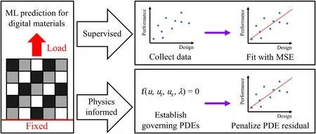
It becomes difficult to explore and understand the material be-haviors of DMs due to the enormous design space.Traditional methods such as experiments and numerical simulations are of-ten hindered by labor or high computational costs.One popular alternative is to use a high capacity machine learning (ML) model (neural network) to interpolate and generalize the entire design space from a sample dataset labeled with experiments or simula-tions [ 14 -17 ].This is also called a supervised ML approach (Fig.1),and has been proven to yield accurate predictions with adequate ground truth data and a properly structured model [ 18 -22 ].On the other hand,data is not the only source of knowledge especially for problems where the well-established physical laws can be en-coded as prior knowledge for neural network training.As seen in Fig.1,such a model is named as the physics-informed neural net-work (PINN) which directly uses the governing equations (typically partial differential equations that define the physical rules) as the training loss rather than learning from data [23] .Researchers have been using PINN as a solution approximator or a surrogate model for various physics problems with initial and boundary conditions as the only labeled data [ 24 -28 ].However,unlike the supervised approach,PINN frameworks must be well engineered to fit dif-ferent problems.For example,Heider et al.[29] successfully rep-resent a frame-invariant constitutive model of anisotropic elasto-plastic material responses as a neural network.Their results show that a combination of spectral tensor representation,the geodesic loss on the unit sphere in Lie algebra,and the“informed”direct relation recurrent neural network yields better performance than other model configurations.Yang et al.[30] build a Bayesian PINN to solve partial differential equations with noisy data.Their frame-work is proved to be more accurate and robustness when the pos-terior is estimated through the Hamiltonian Monto Carlo method rather than the variational inference.Chen et al.[31] realize fast hidden elastography based on measured strain distributions using PINNs.Convolution kernels are introduced to examine the conser-vation of linear momentum through the finite difference method.The above-mentioned works demonstrate the complexity of PINN applications,which thus require intense research work.

Fig.1. A schematic comparing the supervised learning and physics-informed learning for material behavior prediction.A supervised learning approach fits a model to approximate the ground truth responses of collected data.A physics-informed approach fits a model by directly learning from the governing partial differential equation.

In this paper,we will introduce how PINNs can be extended into DM problems by solving the following challenges.First,the material property (e.g.,modulus,Poisson’s ratio) of a DM is described in a discontinuous manner and thus not differentiable over space.Therefore,the PINN approach must be modified to compensate for this DM specific feature.Second,nonlinear strains generated by large deformation on solids should be approximated and constrained properly.Lastly,the proposed PINN should be reasonably accurate and efficient compared with numerical simulations and supervised ML models.This approach can offer a label-free training of ML models to more efficiently understand and design next-generation composites.

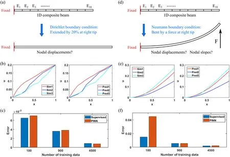
The PINN is first tested on a 1D digital material which is simply a composite beam as seen in Fig.2a.We would like to make a note that all quantities presented in this paper are dimensionless,meaning that one could use any set of SI units as long as they are consistent (e.g.,m for length with Pa for stress,or mm for length with MPa for stress).The beam consists of 10 linear elastic segments which all have the same length of 0.1 but different modulus within a range of 1-5.The beam is fixed at its left tip and extended by 20% on its right tip (Dirichlet boundary condition).The governing equation for this 1D digital material can be easily derived as(Eu’)’=0 whereEdenotes the modulus,udenotes the displacement field,and the material is assumed to be free of body force.For this problem,only the linear component of strain is considered,which will be extended into a nonlinear strain in a later section.Our goal is to train a neural network to predict the displacement field under various material configurations.A normal physics-informed approach would construct a neural net which takes material configurationEand material coordinatexas inputs,and outputs a displacement response at that coordinate.The loss function would simply be the squared residual of the governing equation given above.The auto differentiation packages of ML frameworks allows straightforward computation ofu’by backpropagating the neural network.However,one also needsE’which is not available under a digital material configuration whereEis basically a combination of step functions.

Therefore,instead of the strong governing equation which requires spatial differentiation,a weaker expression is adopted that takes the integral of the material strain energy over space.For this static problem,the solution for a minimum strain energy minualso satisfies the strong form governing equation.Here,we construct a neural network which takes onlyEas the inputs,and outputs the nodal displacement valuesui.The total strain energy is evaluated using a first-order interpolation function for the displacement field which is then passed as the loss function for the neural network.The neural network contains 3 hidden layers of size 10 and uses tanh() as the activation function.900 sets of input features are randomly generated to train the model.200 sets of features are labeled by numerically solving the governing equation where half is used for validation,and the other half for final testing.The model is trained for 50 epochs on the Adam optimizer with a batch size of 10 and a learning rate of 0.001.We stop training at an epoch number where the model performance starts to converge.This stopping criterion is implemented for all the models presented in this paper.The trained PINN shows an average displacement prediction error of 0.0038 for each node based on the testing set.Fig.2b shows a comparison between some predicted shapes of the beam and the ground truth shapes.As a reference,another neural network is trained in a supervised manner with the same dataset but labeled.This supervised model shares the exact same structure and hyperparameter settings,and reaches a testing error of 0.0036 after 50 epochs of training.To examine PINN’s performance under different data density,both models (PINN and supervised) are further trained with 180 and 4500 sets of input features.The same proportion of validation and testing data are labeled for each case.A comparison of performance is shown in Fig.2c where both models produce similar testing errors under different sizes of datasets.So far,we have demonstrated the viability of training a PINN with a strain energy loss for this simple linear digital material under a Dirichlet boundary condition.And it turns out that the same approach also functions properly under a Neumann boundary condition with a few modifications.

Figure 2d shows a same 1D digital material configuration as previous,but subject to a constant force of 1 at the right tip bending the beam upward.The beam is assumed to possess a constant area moment of inertia of 0.6 at its cross section.Again,the minimum energy approach is adopted which has an expression of minvIdenotes the area moment of inertia of the beam cross section,vdenotes the vertical displacement field,andFdenotes the constant force at the right tip.Notice that there is a work term associated with the tip forceFin the system energy expression when there is a Neumann boundary condition.To numerically evaluate the strain energy (the integral term) of a bent beam,we adopt the Hermite shape function [32] which assigns two degrees of freedom at each nodei:the beam deflectionviand beam slopevi,so that the beam smoothness is guaranteed.Therefore,the neural network has an input layer of size 10 to receive the material configurationE,an output layer of size 20 to predict the deflections and slopes at the nodes (except for the left tip which is fixed and has a slope of 0),and 3 hidden layers of size 30.The neural network for the bending problem has more neurons in its hidden layers because it is expected to have larger and more complex output responses.The activation is chosen to be the scaled exponential linear unit function.The model is trained for 80 epochs on the Adam optimizer on 900 sets of randomly generated input features with a batch size of 1 and a learning rate of 0.001.Another 200 sets of features are randomly generated and labeled for validation and testing.

Fig.2. a A 1D digital material extension problem subject to a Dirichlet boundary condition.The goal is to have a PINN predicting the displacement responses based on different material configurations. b Comparison between numerical simulated material deformation and neural network predicted material deformation.Here,“x”represents the coordinate,“u”represents the displacement,“Sim”represents the simulation results and“Pred”represents the model predicted results.c Comparison between the supervised model and the PINN with different amount of data for the 1D tension problem.d A 1D digital material bending problem subject to a Neumann boundary condition.The goal is to have a PINN predicting the deflection responses based on different material configurations.e Comparison between numerical simulated material bending and neural network predicted material bending.Here,“x”represents the coordinate,“u”represents the deflection,“Sim”represents the simulation results and“Pred”represents the model predicted results. f Comparison between the supervised model and the PINN with different amount of data for the 1D bending problem.

The trained PINN shows an average deflection prediction error of 0.0056 for each node based on the testing set.Figure 2e shows a comparison between some predicted shapes of the beam and the ground truth shapes.A reference supervised neural network with the exact same structure and hyperparameters reaches a testing error of 0.0055 after 80 epochs of training.The performance of the PINN and the supervised model is also compared under different sizes of datasets as discussed for the tension problem (Fig.2f).Interestingly,the results of this bending problem have two major characteristics.First,the supervised model greatly outperforms the PINN under a low data density (180 sets of training features).Second,using any batch size other than 1 would greatly reduce the training performance.It is believed that these phenomenons are caused by the work term -Fvtipwhich assigns a much larger gradient on the right tip deflection than any other model outputs.This unbalanced gradient can introduce instability during the parameter descent process which will be explored further in future studies.

The above discussions illustrate the energy-based physicsinformed models for intuitive 1D digital materials.However,realworld problems can be more complex in the following aspects:high order tensor operation for 2D or 3D geometries,nonlinear strain as a result of large deformation,computational efficiency for evaluating and backpropagating the energy loss,which will be addressed below.

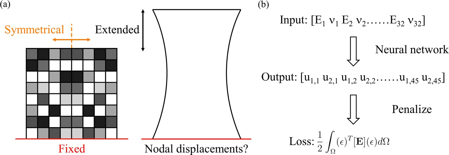
Figure 3a shows a 2D digital material configuration that is symmetrical about its vertical centerline.The material sheet is fixed at its bottom edge and extended by a distance of 3 at its top edge (a Dirichlet boundary condition).The entire material domain is discretized into 8 × 8 elements with a size of 1 × 1.The material elements obey isotropic linear elasticity where the modulusEstays in the range of 1-5,and the Poisson’s ratioνstays in the range of 0.3-0.49.Figure 3b gives a simple illustration of the physicsinformed model for this 2D digital material.Due to the symmetry and boundary conditions,this configuration has a total of 64 features (2 material properties for each of the 32 elements on one side) as the inputs for the neural network,and 90 nodal displacement responses (45 nodes on one side,each has 2 displacement responses) as the outputs of the neural network.Note that there are 23 nodal displacements constrained by the boundary conditions or the symmetry,so the actual prediction should be of size 67.However,we set the output layer size to 90 for a better computational efficiency which will be explained in more details later.The loss function for this neural network is again the elastic energy but in a 2D expression minuHere we use the 2D logarithmic strain vector forεto account for the nonlinearity under large deformation,andErepresents the 3 × 3 2D material stiffness matrix built upon modulus and Poisson’s ratio.The integral is evaluated numerically using 4-point Gaussian quadrature on first-order 2D shape functions.As the problem size and complexity increase,sequentially computing the element strain energy loss would be extremely inefficient and more expensive than directly labeling the data through simulations.Notice that the element strain energies and Gaussian quadrature can both be computed parallelly.Therefore,when implementing the energy loss function,we can greatly accelerate the forward and backward path of the neural network utilizing the batch tensor operation on a GPU.

Fig.3. a A 2D digital material extension problem subject to a Dirichlet boundary condition.The entire 2D sheet has a size of 8 × 8,and is extended by a distance of 3 at its top edge. b A simple schematic showing the structure of the PINN for the 2D digital material.The model takes the modulus and Poisson’s ratio as inputs and outputs the vertical and horizontal displacements for each node.The total material strain energy is used as the loss function for training.

The following discussions will be based on Pytorch,but can be easily extended to other frameworks.First,we pre-construct mask tensors to filter the model outputs so that the displacement predictions will obey the boundary conditions exactly.This masking operation blocks any gradients passing the boundary nodes.The masked output layeruis then reshaped (according to connectivity) into a fifth-order tensor of size batch × 32 × 1 × 2 × 4 where the second dimension represents the 32 elements.The quadrature tensor is also pre-constructed with a size of batch × 1 × 4 × 4 × 2 where the third dimension represents the 4 quadrature points.Using Eq.(1) which multiplies the last two dimensions of the displacement tensor and the quadrature tensor,we can calculate the displacement gradient on the local coordinatesξfor each element at each quadrature point.

Next,the global displacement gradient∂u/∂x(it has a shape of batch × 32 × 4 × 2 × 2) can be obtained by multiplying the local gradient tensor with the mapping tensor fromξtoxwhich is a fixed quantity and can be pre-constructed before training.The deformation gradientFequals to∂u/∂x+IwhereIis a 2 × 2 identity matrix.The Green’s deformation tensorCcan then be calculated asFTFwhich further equals to the square of the right stretch tensorU2.And the nonlinear logarithmic strainεcan be obtained by taking the square root and natural log on the eigenspace ofC(take operations on the eigenvalues ofC,then reconstruct the tensor).The strain tensor is then reshaped into a size of batch × 32 × 4 × 3.

For the material stiffness matrix,the input features are augmented so that instead of passingEandνandνinto the model,we passE/(1 -ν2),Eν/(1 -ν2),andE/[2(1 +ν)] for each material element (the neural network has an input layer of size 96 instead of 64).Thereafter,E(size of batch × 32 × 4 × 3 × 3) can be easily constructed by gathering the corresponding input features on each of its rows without an element-wise value assignment.The strain energy of each element at each quadrature point can now be parallelly computed on GPU through tensor products between reconstructedεandE.The last step is to sum over the second(size of 32) and third (size of 4) dimensions of the energy tensor to obtain the total strain energy as the prediction loss.

Every step discussed above is a pure tensor operation that is parallelable on a GPU and differentiable.However,the deformation gradientFstep may require extra care.Due to the neural network’s ignorance of the physical world,the model is theoretically allowed to predict any displacement responses without constraints at the early stages of training.This can produce physically nonexistentFwhich has a negative determinant.Although the model training can still proceed for such erroneousF,the gradient update for the neural network parameters are likely pointing towards a wrong direction and thus negatively affect the convergence rate and stability.To overcome this issue,one method is to initialize the neural network so that the initial guesses of nodal displacement responses have small magnitudes compared to the size of an element (1 × 1),and the model parameters never enter the problematic region.Another method we adopted is adding this extra term -min(0,J) to the loss function whereJ(Jacobian) is the determinant ofF.This term has no effect on training whenJis positive,but it penalizes and forces the neural network to produce more positiveJvalues whenever it predicts an erroneousF.

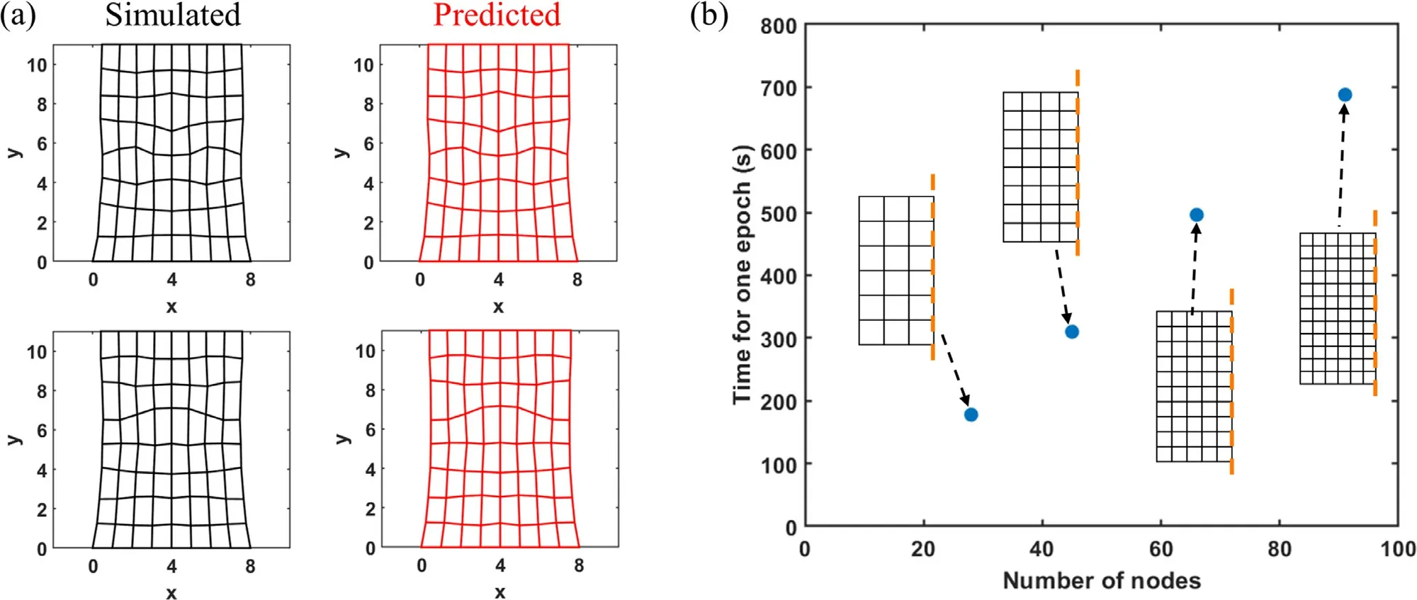
With the above discussions in mind,the PINN for this 2D digital material has an input layer of size 96,an output layer of size 90,4 hidden layers of size (96,128,128,90),and an activation function tanh().The model is trained for 50 epochs on the Adam optimizer on 4500 sets of randomly generated input features with a batch size of 5 and a learning rate of 0.001.Another 1000 sets of features are randomly generated and labeled for validation and testing.The trained PINN shows an average testing error of 0.021(average Rsquared value of 90.48%) for the nodal displacements on each coordinate.Figure 4a shows a comparison between some predicted shapes of the deformed 2D material and the ground truth shapes.A reference supervised neural network with the exact same structure and hyperparameters reaches a testing error of 0.019 after 50 epochs of training.Nvidia RTX 2080 GPU is used to accelerate tensor operations.To further examine the scalability of our energy loss,we construct neural networks for different mesh configurations as seen in Fig.4b.The neural network size scales linearly with the number of nodes.All these models with different sizes are each trained on 4500 sets of randomly generated input features for one epoch.The corresponding real-world time is plotted in Fig.4b which scales linearly with respect to the number of nodes.Due to the nonlinearity and stochasticity of the neural network training process,it is difficult to bound the required number of epochs till convergence and will be explored in future work.However,the results still show the potential of the energy-based PINN to be more efficient than generating simulation labels (simulation cost is typicallyO(n2)-O(n3) wherenrepresents the number of nodes [33]).

Fig.4. a Comparison between numerically simulated material deformation and neural network predicted material deformation for the 2D digital material.b Computation cost of one epoch of model training under different mesh.The orange dashed lines indicate the symmetry axis.

In summary,we successfully trained PINN models for DM using the minimum energy criteria instead of the governing equation as the loss function.The method shows comparable accuracy to the supervised models on the 1D tension,1D bending,and 2D tension problems discussed in this paper.Results show that our proposed PINN can properly approximate the logarithmic strain and fix any erroneous deformation gradient by adding a hinge loss for the Jacobian.Moreover,the loss evaluation step can be parallelized over the elements and quadrature points on a GPU through proper tensor rearrangements on input features and outputs responses.The single epoch computation cost of the optimized algorithm scales linearly with respect to the number of nodes (or elements) in a DM mesh.This work shows the possibility of training PINNs for digital materials accurately and efficiently,allowing direct ML exploration of next-generation composite design without the necessity of expensive multi-physics simulations.

Acknowledgements

The authors acknowledge support from the Extreme Science and Engineering Discovery Environment (XSEDE) at the Pittsburgh Supercomputing Center (PSC) by National Science Foundation grant number ACI-1548562.Additionally,the authors acknowledge support from the Chau Hoi Shuen Foundation Women in Science Program and an NVIDIA GPU Seed Grant.