Ergodic sensitivity analysis of one-dimensional chaotic maps

2020-12-13AdamliwiakNishaChandramoorthyQiqiWang

Theoretical & Applied Mechanics Letters 2020年6期

Adam A. Śliwiak*, Nisha Chandramoorthy, Qiqi Wang

a Department of Aeronautics and Astronautics, Massachusetts Institute of Technology, Cambridge, MA 02139, USA

b Center for Computational Science and Engineering, Massachusetts Institute of Technology, Cambridge, MA 02139, USA

c Department of Mechanical Engineering, Massachusetts Institute of Technology, Cambridge, MA 02139, USA

Keywords:Sensitivity analysis Chaotic systems Ergodicity Space-split sensitivity (S3) method

ABSTRACT Sensitivity analysis in chaotic dynamical systems is a challenging task from a computational point of view. In this work, we present a numerical investigation of a novel approach, known as the space-split sensitivity or S3 algorithm. The S3 algorithm is an ergodic-averaging method to differentiate statistics in ergodic,chaotic systems,rigorously based on the theory of hyperbolic dynamics. We illustrate S3 on one-dimensional chaotic maps, revealing its computational advantage over naïve finite difference computations of the same statistical response.In addition,we provide an intuitive explanation of the key components of the S3 algorithm, including the density gradient function.©2020 The Authors. Published by Elsevier Ltd on behalf of The Chinese Society of Theoretical and Applied Mechanics.This is an open access article under the CC BY-NC-ND license (http://creativecommons.org/licenses/by-nc-nd/4.0/).

Sensitivity analysis is a discipline that studies the response of outputs of a certain model to changes in input parameters. It involves computing the derivatives of output quantities of interest with respect to specified parameters. This mathematical tool is essential in many engineering and scientific applications, as it enables optimal design of structures [1,2] and fluid-thermal systems [3], analysis of heterogeneous flows [4], supply chain management [5], estimate errors and uncertainties in measurement,modeling and numerical computations [6,7]. A classic example from fluid mechanics is a turbulent flow past a rigid object, in which the sensitivity of the drag (resistance) forces with respect to the Reynolds number and other flow parameters [8,9], is of interest. Particularly, aerospace engineers use the computed sensitivity in the design of airfoils [10]. This mechanical phenomenon is governed by a strongly nonlinear dynamical system and,moreover, it features an extra difficulty, namely the chaotic behavior.

Computing such sensitivities in chaotic dynamical systems is a challenging task. The primary issue is the so-calledbutterfly effect, which is a large sensitivity of the system to initial conditions.This concept is associated with the classical study of Edward Lorenz on climate prediction [11]. Quantitatively, it means that any two points initially separated by an infinitesimal distance diverge at an exponential rate. This implies the prediction of farfuture states in chaotic phenomena is hardly possible. We observe this phenomenon in daily weather forecasts, as the predictions of several weeks forward tend to be highly inaccurate.However, we are sometimes interested in predicting the response of long-time averaged behavior, to perturbations [8,9,12].

In the last few decades, there have been different attempts to compute sensitivities of long-term averages in chaotic systems.The conventional methods [13,14], which require solving either tangent or adjoint equations, fail if the time-averaging window is large. Due tobutterfly effect, almost every infinitesimal perturbation to the system expands exponentially, and therefore the sensitivity computed using the tangent or adjoint solutions grows equally fast. A more successful family of methods utilize the concept of shadowing trajectories [15–17]. However, shadowing methods have been proven to have a systematic error,which can be non-zero if the connecting map between the base and shadowing trajectory is not differentiable [18]. Some approaches adopt the Fluctuation-Dissipation Theorem, which is widely used in the statistical equilibrium analysis of turbulence,Brownian motion, and other areas [19]. Unfortunately, they are inexact as well, when they do not assume specific properties of the physical systems, e.g. Gaussian distribution of the equilibrium state [20]. Moreover, they require solving costly Fokker-Planck equations, which makes them infeasible for large systems [21]. Another group of methods for sensitivity analysis are trajectory-based and utilize Ruelle's linear response formula[22]. Many of these techniques, generically referred to as ensemble methods, solve tangent/adjoint equations and compute ensemble average over a trajectory to estimate the sensitivity[23,24]. The two major drawbacks of ensemble-based methods is that they exhibit slow convergence since they suffer from exponentially increasing variance of the tangent/adjoint equations[12,23].

Space-split sensitivty (S3) is an alternative trajectory-based method that uses Ruelle's formula [25]. However, unlike the ensemble methods, it does not manifest the problem of unbounded variances. Moreover, the S3 method does not assume that the probability distribution in state space is of a particular type(e.g. Gaussian), and also does not rely on directly estimating the probability distribution by e.g. discretizing phase space. In the paper, we will closely review the basic concepts of the S3 method in the context of one-dimensional chaotic maps.

We introduce two families of perturbed one-dimensional chaotic systems that can generally be expressed as

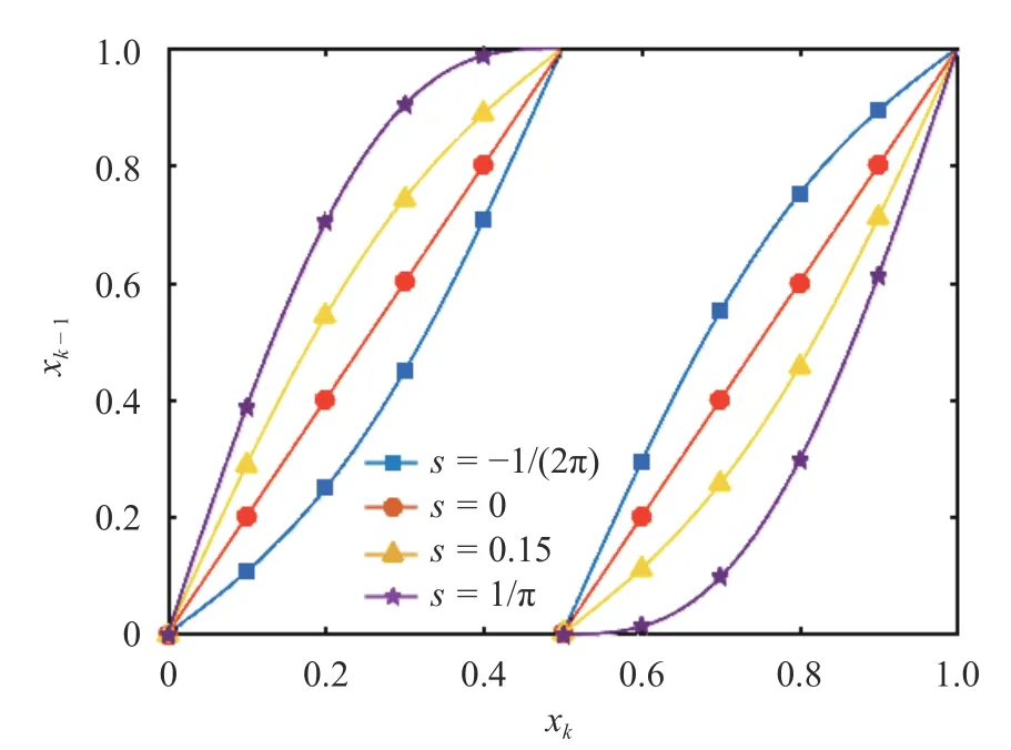
Fig. 1.The sawtooth map at different values of parameter s. Note if we obtain the classical Bernoulli shift

wherexinitis a given initial condition, whilesdenotes a scalar parameter. LetJbe a scalar observable. Our quantity of interest is the infinite-time average orergodicaverage ofJ,

In particular, we focus on the relationship between〈J〉and the parametersforφ. In addition, we review the concepts of Lyapunov exponents and ergodicity through numerical illustrations on the two maps.

We consider as our first example, perturbations of the sawtooth map, also known as the dyadic transformation, defined in the following way:

It is a periodic map that maps [0 ,1) to itself. Figure 1 illustrates the sawtooth map for different values of the parameters.

A natural question that arises is whether the chosen is map actually chaotic. Roughly speaking, achaoticmap shows high sensitivity to initial conditions. For example, considers=0, and two phase pointsxandx+δx. Under one iteration of the map,these two points are now separated by a distance of 2δx. Thus, in the limitδx→0,a trajectory that is infinitesimally separated fromxatn=0 moves away from the trajectory ofxat an exponential rate of l og 2≈0.693. This exponential growth of perturbations to the state is the signature of chaotic systems and is measured by the rate of asymptotic growth, known as the Lyapunov exponent (LE) and denoted byλ. More rigorously, the Lyapunov exponent is defined by

which clearly indicates that the infinite-time averaged rate of growth converges to a constant. We say that a map is chaotic when its LE is positive. Eq. (4) requires computing the derivative of the map at points along a trajectory. Note that the value of the Lyapunov exponentdoesnot depend oninitialconditionxinit ,nor onthestepk.Figure2 showsthatλ>0foralls∈(−1/(2π),1/π]meaning that the sawtooth map is chaotic in this regime. This can be easily justified by the observation that∂φ/∂x≥1for allx∈[0,1], whensis in this regime.

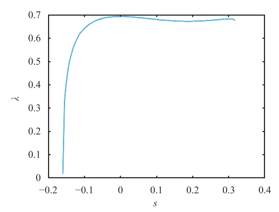
Fig. 2. Relation between the Lyapunov exponent λand parameteror the sawtooth map

In case of the classical Bernoulli shift, i.e. whens=0, a repetitive application of the sawtooth map always appears to converge to a fixed point when simulated numerically. This is because all machine-representable numbers with a fixed number of digits after the binary point are dyadic-rational numbers,which converge to the fixed point 0 under this map, because the sawtooth map ats=0 is simply a leftshift operation on binary digits. More details about this problem and possible remedies can be found in A. Note also that ifs=0 andxinitis rational, the forward orbit ofxinitwould either converge to a fixed point or be periodic, containing a finite number of distinct values within the interval [0 ,1). For example, ifxinit=0.1, then all future states belong to a four-element set, { 0.2,0.4,0.6,0.8}, andxk=xk+4for allk>0. This is an example of an unstable periodic orbit; in this paper, we are interested in chaotic orbits, which are aperiodic and unstable to perturbations.

Another example of a chaotic map is the cusp mapφ:[0,1]→[0,h] defined as follows,

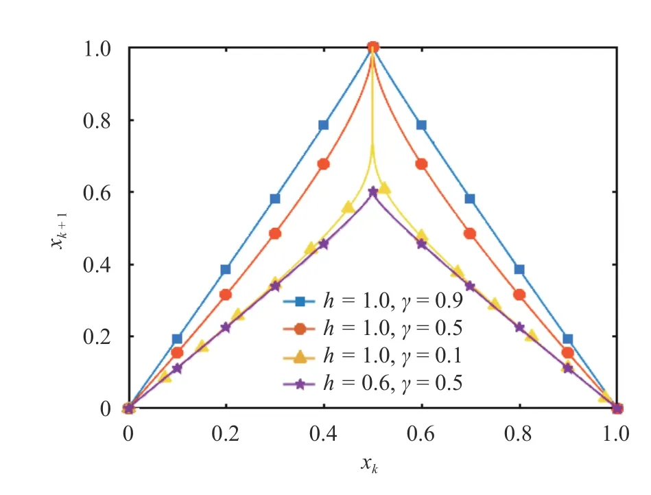
Fig. 3.The cusp map at different values of parametersh and γ.Note all the curves include points ( 0,0)and ( 1,0), while the tip is located at ( 0.5,h). If h =γ=1, the map is piecewise linear, and this particular case is usually referred to as the tent map

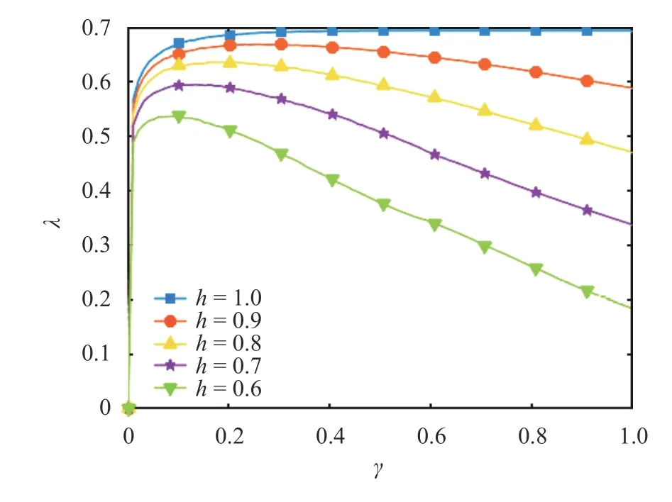
Fig. 4.Relation between the Lyapunov exponent λ and parameter γ∈[0,1]for the cusp map

The above function produces a spade-shaped graph, as shown in Fig. 3.

The cusp map is a two-parameter map withs={h,γ}, wherehis the height, whileγis a parameter that determines the sharpness of the tip. We use the definition Eq. (4) to compute the LE of the cusp map at different values ofhandγ. From the positivity of the Lyapunov exponent shown in Fig. 4, we see that the cusp map is always chaotic ifγ∈[0,1] andh≥0.6.

Historically, the cusp map has been used as a one-dimensional representation of the three-dimensional Lorenz'63 system [11], a set of ordinary differential equations used as a model for atmospheric convection. Specifically, the iterates of the cusp map are local maxima of the third coordinate of the Lorenz'63 system [26].

The long-time average of the objective function,〈J〉, was calculated using 100 million iterates of the map, with the initial condition chosen uniformly, at random between 0 and 1, in the following way:

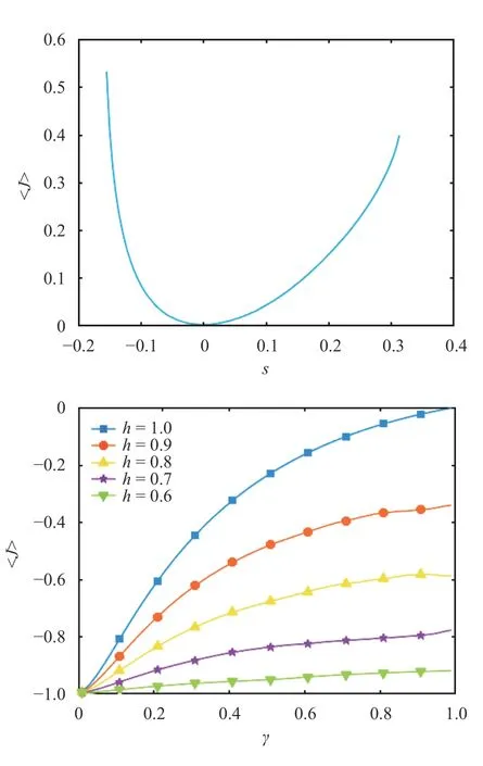
Fig. 5.Long-time averaged behavior with respect to the map parameter for the sawtooth (upper plot) and cusp map (lower plot). The objective function itself does not depend to the parameter, and is defined as J (x)=cos(2πx). In our computations, J is averaged over 100 million samples

wherexi+1=φ(xi). We choose a sufficiently largeNto ensure that the right hand side converges to a fixed value, within numerical precision. Figure 5 illustrates examples of the mean statistics (i.e. long-time averages) and their dependence on the map parameters for both the sawtooth and cusp map.

In the computation of the long-time averages of the objective function, we used the concept of ergodicity. This property guarantees that long-time averages do not depend on the initial conditions. That is, the time average of the objective function(right hand side of Eq. (6)) converges, asN→∞, to a value independent of the initial conditionx0, for almost everyx0chosen uniformly between 0 and 1. This limit equals the expected value of the same objective function over an ensemble of initial conditions distributed according to anergodic,invariantprobability distribution ρ. This probability distribution ρ is invariant under φ,in the sense that for any open intervalA⊂(0,1),ρ(A)=ρ(φ−1(A)).In addition, ρ is defined by the fact that expectations with respect to ρ are the same as infinite-time averages starting from a point uniformly distributed in the unit interval.Such a probability distribution ρ,is known as the Sinai–Ruelle–Bowen (SRB) distribution [27], and only sometimes coincides with the uniform distribution (it does e.g. for the sawtooth map ats=0). The above description can be mathematically rephrased as follows, for almost everyx0uniformly distributed in ( 0,1),

Thus, in ergodic systems, there exist two alternative ways of computing the long-time average, either through the averaging of the time-series or ensemble averaging. The latter requires prior computation of the probability distribution, which will be explained and illustrated in the next sections. Using these preliminary concepts, we will review the space-split sensitivity method to compute the derivative of 〈J〉 with respect to the map parameter.

In Ref. [22], Ruelle rigorously derived a formula for the derivative of the quantity of interest, 〈J〉, with respect to the map parameters. This expression is an ensemble average (or expectation)with respect to ρ, which can be simplified for one-dimensional maps φ :U→Uto

where

reflects the parameter perturbation of the map, whileUrefers to the unit interval [0,1). A direct evaluation of Eq.(8)is computationally cumbersome for the following reason. Notice that the integrand of the right hand side of Eq. (8) involves a derivative of the composite function that can be expanded using the chain rule to the form

As discussed earlier, for a largek, the product of the derivatives exponentially grows withk. However, Ruelle's series converges due to cancellations of these large quantities, upon taking an ensemble average. This problem makes the direct evaluation of Ruelle's formulation computationally impractical since a large number of trajectories are needed for these cancellations. More precisely, since for a largek,

at almost everyx, we need to increase the number of trajectories by a factor of O (e2λk) in order to reduce the mean-squared error in a linear fashion. For example, consider the sawtooth map withs∈[−1/(2π),1/π]. In this case,(∂φ/∂x)∈[1,4]. One can easily verify that even for moderate values ofk, an overflow error is encountered. Another challenge is that the evaluation of the SRB distribution requires expensive computation of map probability densities [21]. In a recent study [25], Ruelle's formula has been reformulated to a different ensemble average, known as the S3 formula. In that work, the latter formula has been derived for maps of arbitrary dimension, and is based on splitting the total sensitivity into stable and unstable contributions. Note the notion of splitting the perturbation space is irrelevant for 1D maps, and the one-dimensional perturbation is, by the definition of chaos, unstable. Therefore we will skip some aspects of the original derivation, and note that our derivation represents only the unstable component of sensitivity in Ref. [25]specialized to 1D.

The S3 formula, corresponding to Eqs. (8)–(9), can be expressed as follows:

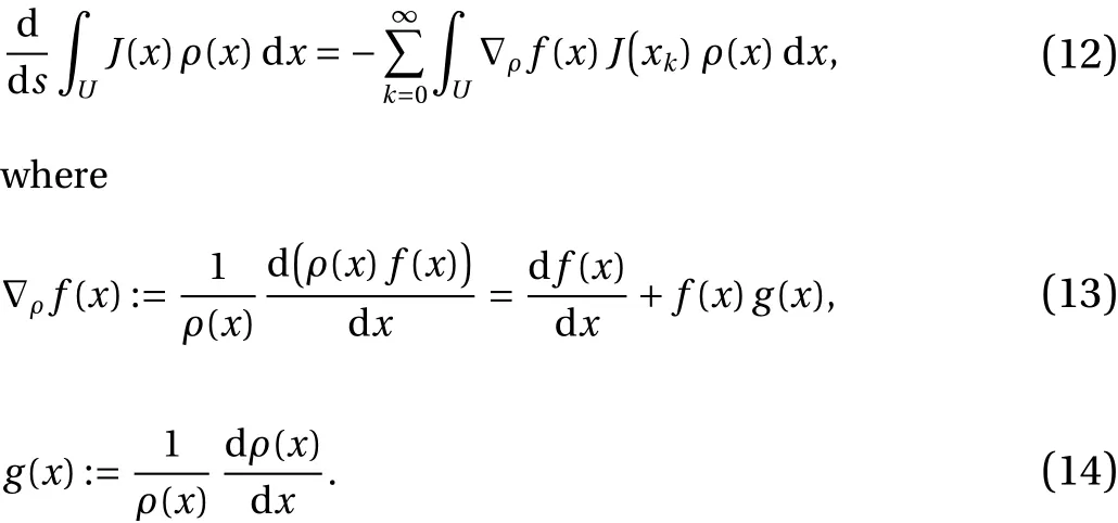
For one-dimensional maps, the derivation is simple, as it requires integrating Eq. (8) by parts and the fact that the integral of df/dxat the boundary ofUvanishes; see B for the full derivation. We observe that bothJand df/dxhave their analytical forms. However, the functiong(x), which will be referred to asdensity gradient, does not have a closed-form expression, since the SRB distribution ρ is unknown. The density gradientgrepresents the variation in phase space of the logarithm of ρ (x),

In the next section, we focus on further interpretingg(x), its computation and verification on the 1D maps introduced.

We focus on the density gradient function, denoted byg(x).First, we present a computable, iterative scheme forg(x).Moreover, we provide an intuitive explanation forg(x) and visualize it on the maps introduced.

Based on the S3 formula (Eq. (12)), we can conclude the recursive relation

holds. The full derivation of Eq. (16) is included in Appendix C.This recursive procedure can be used to approximateg(x) along a trajectory in the asymptotic sense, which means that we need a sufficiently large number of iterations to obtain an accurate approximation ofg(x) [25]. In practice, we generate a sufficiently long trajectory, compute first and second derivatives of the map evaluated along the trajectory, and apply Eq. (16). We arbitrarily setg(xinit)=0, to start the recursive procedure, and obtaing(φ(xinit)).The recursion is continued by settingx=φ(xinit), and so on. For a sufficiently largeK, the true value ofg(φK(xinit)) is approached, for almost every initial conditionxinit.

To intuitively understand the density gradient formula (Eq.(16)), we isolate the effects of each term in Eq. (16). In order to do this, we consider a small interval around an iteratexkand examine two cases: (1) the map is a straight line on this interval and (2) the map has a constant curvature on this interval. These two cases are graphically shown on the left (numbered as 1) and right (numbered as 2) hand sides of Fig. 6. Thex-axis represents an interval around an iteratexk, and they-axis an interval aroundxk+1=φ(xk). The densityρ, around each interval, is shown adjacent to the axes, as a colormap. The colors reflect the distribution ofρon a logarithmic scale.

1. Consider a small region of (x−ϵ,x+ϵ) where the mapφ(x)has zero second derivative, i.e., the first derivative dφ/dxis constant. As shown in Fig. 6a, let us assume that the density on the left side of the region,ρ(x−ϵ), is higher than the density on the right side,ρ(x+ϵ). Due probability mass conservation, the mapped density can be calculated using the following equation,

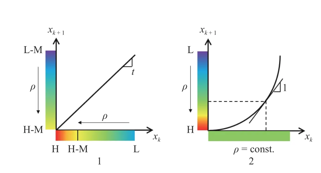
Fig. 6.A graphical representation of two different scenarios in onedimensional maps,to intuitively understand the derivation of the quantity g.The bold lines illustrate the map, while shaded bars adjacent to each axis represent the corresponding density distribution on that axis. The region around H corresponds to a high value of density, while the region around L to low values. The slope of the line is indicated as t

Since we consider case dφ/dx>0, we drop the absolute value.On this interval where the map is a straight line, this statement says that the density aroundφ(x) is a constant multiple of the density aroundx. On the logarithmic scale, the density aroundφ(x)is shifted by a constant, when compared to the density aroundx, since

This relationship is graphically depicted in Figure 6a, where the regions markedHandL, corresponding to higher and lower densities, are shifted to the left. Notice that Eq. (18) implies that the difference, on the logarithmic scale, between the higher and lower densities on they-axis equals the difference between the higher and lower densities on thex-axis. However, the small interval is stretched by a factor of dφ/dxunder one iteration of the map. Thus, the derivative of the logarithm of density decreases by a factor of dφ/dx. Mathematically, we can see this by differentiating both sides of the equation with respect tox(and using that dφ/dxis constant),

From the definition ofg, this reduces to

which is confirmed by our formula, Eq.(16), by setting d2φ/dx2=0.

2. To isolate the effect of curvature of the map ong, we consider a curved map and a constant density region. Thus, by definition,g(x) vanishes in the interval considered. We now describe thatg◦φ(x) becomes non-zero on this interval due to the curvature of the map. Note that Eq. (18) still applies, since it is a restatement of probability mass conservation. This means thatρis reduced by a factor equal to the slope of the map at every point. This is graphically depicted in Fig. 6, in which we have assumed that dφ/dxis an increasing function that crosses the value 1 at the point indicated using dashed lines. To the left of this point, the density is therefore increased (shown asH)aroundφ(x) and to the right, the density is decreased (shown asL), when compared to its uniform value aroundx. Note also the larger the first derivative of the map, the lower the density on they-axis. Again, by taking the derivative of Eq. (18) with respect tox, and using the definition ofg, we obtain

As mentioned in Case 1, the first derivative ( dφ/dx)(x) gives the factor by which a length dxaroundxis stretched (or compressed) byφ. The second derivative gives us the change of this stretching (or compression) as a function ofx. Thus, the effect of a non-zero second derivative is felt by thederivativeof the density, and can again be derived from measure preservation or probability mass conservation.

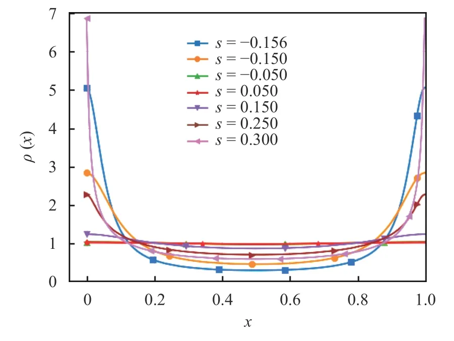
Fig. 7.The plot shows the empirically estimated stationary probability distributions achieved by the sawtooth map (Eq. (3)). Every curve was generated using 125,829,120,000 samples and counting the number of solutions in each of 2048 bins of equal length in the interval[0,1)

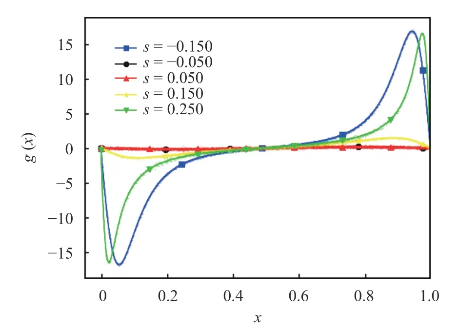
Fig. 8.Density gradient function, g (x) (solid lines), generated using Eq. (16) and compared against the empirically computed value of g (x) (dots), where the derivative of ρ (x)is estimated using finite difference

Then we show numerical results of the density gradient procedure in two examples, the sawtooth and cusp maps, which were introduced in Eqs. (3) and (5) respectively. Figure 7 shows the stationary probability densities of the sawtooth map at different values ofs.

We observe that all curves appear differentiable, however their derivatives are large, near the interval boundaries, whensis close to−1/(2π) or 1 /π. In Fig. 8, we show the distribution of the (averaged) density gradient function,g(x), computed using Eq. (16), at different values ofs, and compare it against its finite difference approximation:[log(ρ(x+ϵ))−log(ρ(x−ϵ))]/(2ϵ).

Note that the expected value of the density gradient is always zero since

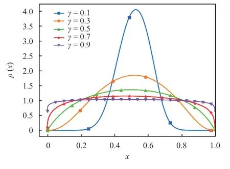
Fig. 9.The plot shows the empirically estimated stationary probability distributions achieved by the cusp map(Eq. (5)), at h =1 and the indicated value of γ. All curves were generated in the same fashion as for the sawtooth case

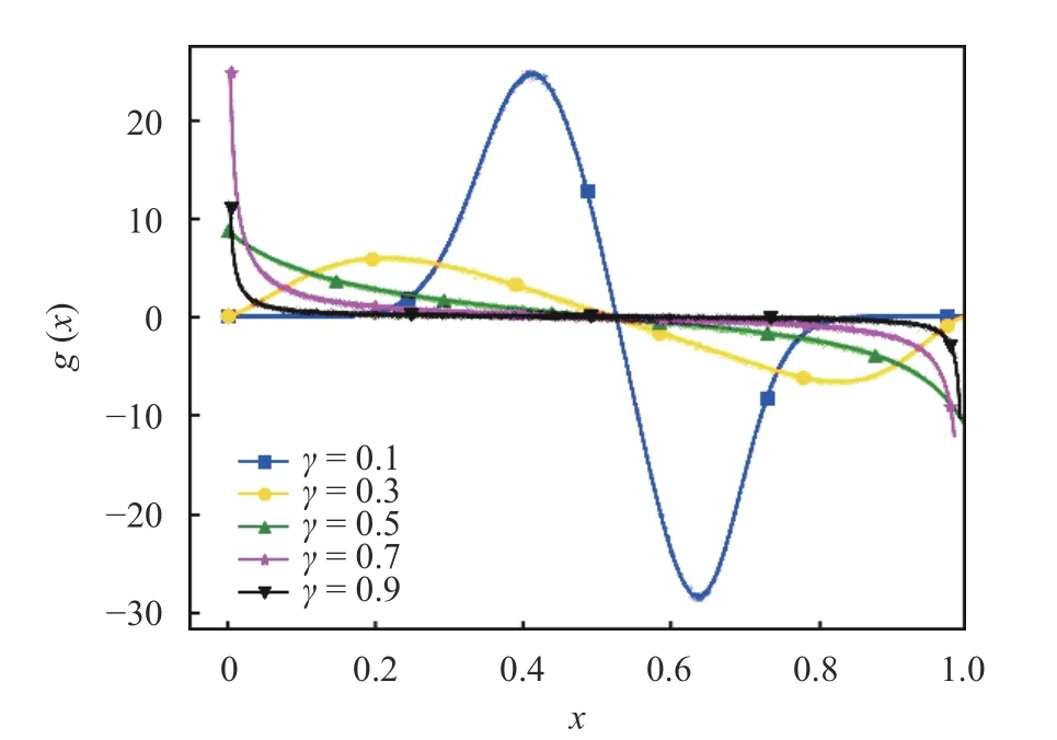
Fig. 10. The plot compares g (x) (solid lines) against the derivative of the empirically estimated stationary probability distributions(dots)achieved by the cusp map (Eq.(5)), at h =1 and indicated value of γ. All curves were generated in the same fashion as for the sawtooth case

We repeat a similar experiment for the cusp map, whose results are presented in Figs. 9 and 10.

We observe a behavior similar to the sawtooth map. Similar to the sawtooth density, the densities computed for the cusp map appear to be differentiable over a range of the parameterγ.However, asγgets close to 1, the densityρ(x) acquires large derivatives at the boundaries of the interval. The boundedness of dρ/dxis needed for the computation ofg(x) to be well-conditioned.

The evaluation of Eq. (12) is the main focus of this paper. In practice, expectations with respect toρ, or ensemble averages,are computed by time-averaging on a single typical trajectory. As mentioned earlier, a time average converges to the ensemble average of the function, as the length of the trajectory approaches infinity. Thus, Eq. (12) can be written as follows, replacing the ensemble averages with ergodic averages

wherexi=φi(xinit)is the point at timei, along a trajectory starting at a typical pointxinit. Using the definition ofg, and taking a long trajectory,

To numerically verify Eq. (24), we consider a set of objective functions, each of which is an indicator function denoted byδc,and defined such that its value is a constant 1 in a small interval aroundcand zero everywhere else on the unit interval. Note every Riemann-integrable function can be approximated, to arbitrary precision, by linear combinations of such indicator functions. With this particular choice, Eq. (24) gives us the gradient of the probability density, since

Thus, by varying the constantcin the interval [ 0,1), and using the density gradient computed using Eq. (15), one can compute dρ/dsover the unit interval by using Eq. (24). This can be compared with the finite difference approximation of dρ/dsgenerated using slightly perturbed values ofsand approximating the density empirically. These estimates can then be used to calculate the derivatives of any other function with a differentiable statistics, using numerical quadrature. The choice of indicator functions exhibits yet another advantage of the S3 method over Ruelle's formula (Eq. (8)). The former is also applicable to objective functions that have non-differentiable points, since unlike a direct evaluation of Ruelle's formula, the derivative ofJ(x)is not used. Figure 11 shows numerical results for the cusp map, in which the density gradient is computed using the spacesplit formula (Eq. (24)) and compared with the central difference derivative.

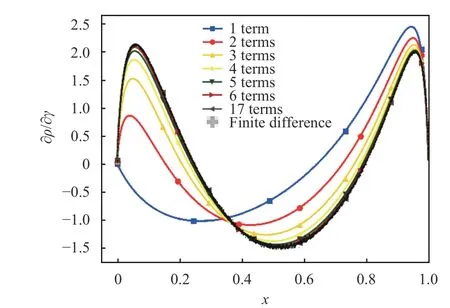
Fig. 11.Sensitivity of the density of the cusp map with respect toγ at h =1,γ=0.5. The solid lines represent the result of Eq. (12) when a finite number of terms is used in the summation over k. The solid line marked with (◁) represents Eq. (12) evaluated with 17 terms,which is visibly indistinguishable from the same series summed over 6 or more terms.The dots represent the finite difference derivative of t he dens i t y, eval uat ed based on t he empi r i cal dens i t y at h=1,γ=0.505and at h =1,γ=0.495. Each quantity is evaluated with 125,829,120,000 samples

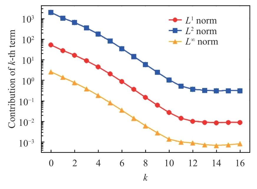
Fig. 12.Contributions from the k -th term to Eq. (12) for the cusp map. Later terms are overwhelmed by statistical noise

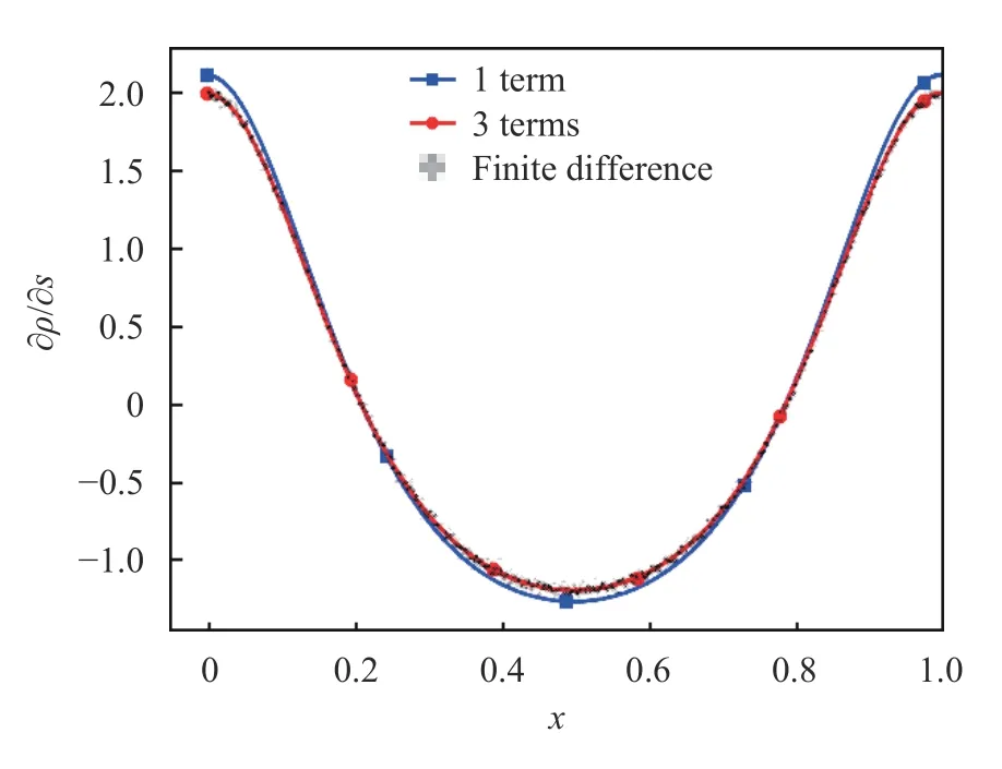
Fig. 13.Sensitivity of the density of the sawtooth map with respect to s at s =0.1. The solid lines represent the result of Eq. (12) when a finite number of terms is used in the summation over k. The solid line marked with (△) represent Eq. (12) evaluated with 3 terms, is aligned with the the finite difference derivative of the density, evaluated based on the density at s =0.105and at s =0.095. Each quantity is evaluated with 125,829,120,000 samples

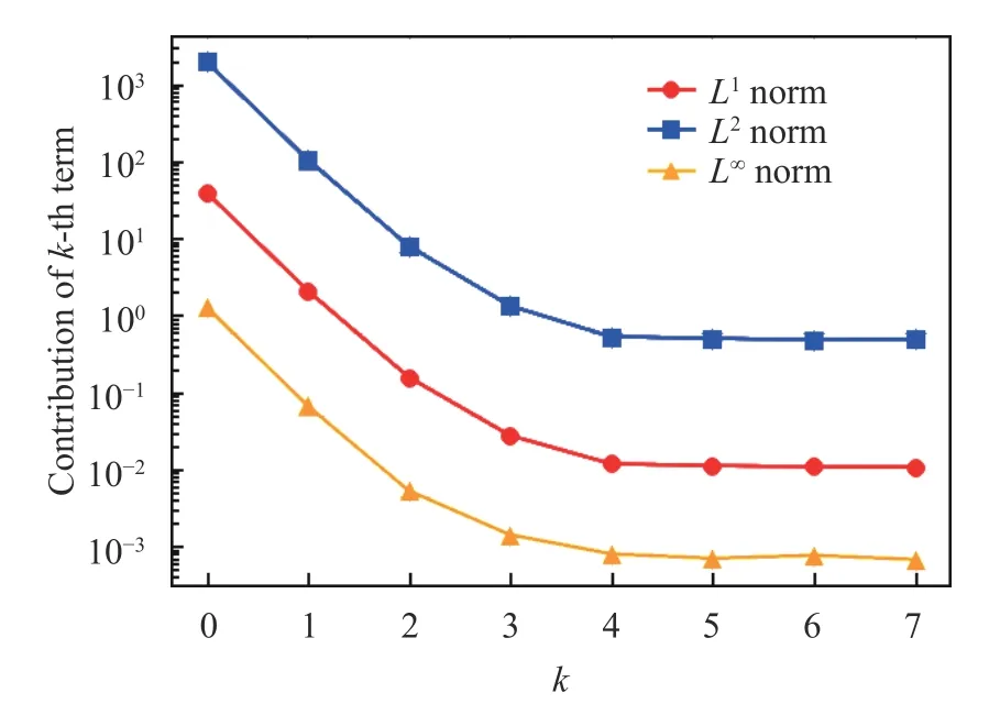
Fig. 14.Contributions from the k -th term to Eq. (12), for the sawtooth map. Later terms are overwhelmed by statistical noise

We observe that only a few terms of the series are required to produce accurate sensitivities. Figure 12 clearly indicates that the consecutive terms of the series in Eq. (23) exponentially decay in norm.

We repeat a similar experiment for the sawtooth map (see Figs. 13 and 14).

In this case, we only need three terms of Eq. (24) to obtain a result that is indistinguishable from its finite difference approximation. The consecutive terms of Eq. (24) also decay exponentially in norm.

Note that each term of Eq. (12) is in the form of a lag-ktime correlation between∇ρfandJ. We use the term "lag-k" as∇ρfand the objective function are evaluated at two different states that areksteps apart. In mixing systems, the lag-ktime correlations converges to zero ask→∞. Moreover, for a family of dynamical systems known as Axiom A, the rate of decay of time correlations is proven to be exponential [27]. In the case of onedimensional maps, Axiom A systems are the ones in which the derivative of the map is different than 1 everywhere. All the map examples we consider in this paper satisfy this requirement. This guarantees that only a small number of time correlation terms are needed to secure high accuracy of the sensitivity approximation.

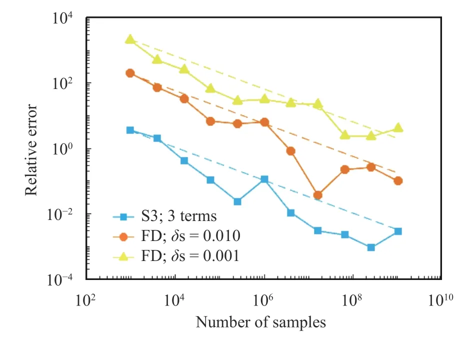
Fig. 15.Relative error of the space-split and finite difference methods as a function of the trajectory length. We compute the parametric derivative of density of the sawtooth map at s =0.1on the left boundary ( x=0) . For the S3 computation (curve marked with (□)),we consider only first three terms of Eq. (12), which corresponds to the line marked with (○) in Fig. 13. For the finite difference approximation,we calculate densities ats=0.105,0.095(curve marked with (□)) and s =0.1005,0.0995(curve marked with (△)). We also computed the S3 approximation using 125,829,120,000 samples and 9 terms of Eq. (12), which serves as a reference value. The dashed lines are proportional to the inverse of the square root of the number of samples

Finally, we compare the space-split sensitivity and classical finite difference method in terms of computational efficiency.Figures 15 and 16, generated respectively for the sawtooth and cusp maps, clearly indicate that the S3 method outperforms its competitor. We observe that the former requires a few orders of magnitude fewer samples to guarantee a similar error.

This is a very promising observation in the context of analysing higher-dimensional systems, since the large cost of generating very long trajectories can make such computations infeasible. Note in the case of both the S3 and finite difference methods, the error is upper-bounded as follows [25],

whereNdenotes the number of samples, whileCis some positive number. This means we observe a convergence rate of a typical Monte Carlo simulation in both methods. However, the factorCis substantially larger in case of finite differencing.Moreover decreasing the step size (indicated asδs) in the finite difference calculation, worsens the accuracy, due the dominance of statistical noise.

We demonstrate a new method to compute the statistical linear response of chaotic systems, to changes in input parameters.This method, known as space-split sensitivity or S3, is used to compute the derivatives with respect to parameters of the longtime average of an objective function. In the S3 method, a quantity calleddensity gradient, defined as the derivative of the log density with respect to the state, is obtained using a computationally efficient ergodic averaging scheme. An intuitive explanation of this iterative ergodic averaging scheme, based on probability mass conservation, is discussed in this paper. The density gradient plays a key role in the computation of linear response.Specifically, the sum of time correlations between the density gradient and the objective function partially determines the derivative of the mean statistic of the objective function with respect to the parameter. The computational efficiency of the S3 formula when compared to finite difference, which requires several orders of magnitude more samples, stems precisely from this new formula to efficiently estimate the density gradient.

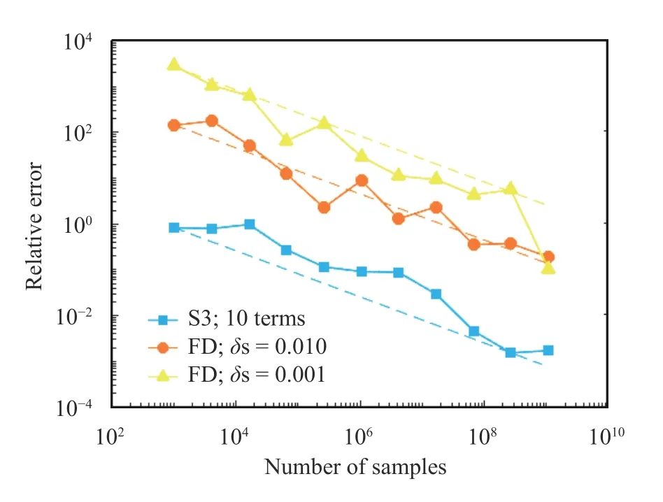
Fig. 16.Relative error of the space-split and finite difference methods as a function of the trajectory length. We compute the parametric derivative of density of the cusp map at h =1, γ =0.5 in the middle of the domain U (x =0.5). For the S3 computation (curve marked with (□)), we consider first ten terms of Eq. (12).For the fini t e di f f er ence approxi mati on, we cal cul at e densi t i es at γ=0.505,0.495(curve marked with (○)) andγ=0.5005,0.4995(curve marked with (△)). We also computed the S3 approximation using 125,829,120,000 samples and 17 terms of Eq. (12), which serves as a reference value. The dashed lines are proportional to the inverse of the square root of the number of samples

In this work, we restrict ourselves to expanding maps in 1D,which are simple examples of chaotic systems. These examples nevertheless give rich insight into chaotic linear response, and specifically into the behavior of the density gradient. Our study shows that in same cases the derivative of the density gradient might be very large, which corresponds to heavy tailedness of the density gradient distribution. This phenomenon, as well as its implication for analysis of higher-dimensional maps, is the main topic of our future work.

Acknowledgement

This work was supported by the Air Force Office of Scientific Research (Grant FA8650-19-C-2207).

Appendix A. Binary floating point problem in simulating 1D maps

Consider the cases=0, Eq. (3) can be compactly expressed using the modulo operator,i.e.xn+1=2xnmod 1. It means we multiplyxnby 2and ifxn+1>1,then we also subtract 1.Using floating point arithmetic, we will observe that there existN>0 such thatxn=0 for alln≥N,which contradicts the assumption of chaotic behavior. This phenomenon is due to the round-off errors associated with the modulo operator. To circumvent this problem, one can change the divisor parameter (of the modulo operation) from 1 to1−ϵ, where ϵ is a small number, e.g.ϵ=10−6. Another possible (and simple) workaround might be a change of variables such that the domain of the new variable has irrational length. Note this approach would also require a modification of the objective function.

Appendix B. Derivation of the S3 formula for 1D maps

In this section, we will show Eqs. (8) and (9) are equivalent to Eqs. (12)–(14). Throughout this derivation we will use a shorthand notation for the compositionv◦φk=vk, wherevis some scalar function defined onU=(0,1), whilekis some integer. Ifk=0, the subscript is dropped. First, note

Integrate the first term of Eq. (27) by parts,

whereUL=0 andUR=1 correspond to the left and right boundary ofU, respectively. Since the domain is periodic, the first term of Eq. (28) vanishes. Thus, we can combine Eqs. (27)and (28) to conclude that

Appendix C. Derivation of the iterative procedure for g in 1D maps

The purpose of this section is to derive the iterative procedure to calculate the density gradientg. We use the same notational convention as in Appendix B. Let us consider a functionhthat is integrable inU=(0,1) and vanishes atUL=0 andUR=1. Using the definitiong=(1/ρ)(∂ρ/∂x), and integrating by parts, we obtain

The key property used in this derivation is the density preservation of φ. We say that the map φ is density-preserving with respect to the density ρ, if for any scalar observablef,holds for any integerk. This implies the left hand side of Eq. (30) can be expressed as