Spatial artificial neural network model for subgrid-scale stress and heat flux of compressible turbulence

Chenyue Xie, Jinchun Wng*, Hui Li, Minping Wn Shiyi Chenc

a Shenzhen Key Laboratory of Complex Aerospace Flows, Center for Complex Flows and Soft Matter Research, Department of Mechanics and Aerospace Engineering, Southern University of Science and Technology, Shenzhen 518055, China

b School of Power and Mechanical Engineering, Wuhan University, Wuhan 430072, China

c State Key Laboratory of Turbulence and Complex Systems, Peking University, Beijing 100871, China

Keywords:Compressible turbulence Large eddy simulation Artificial neural network

ABSTRACT The subgrid-scale (SGS) stress and SGS heat flux are modeled by using an artificial neural network(ANN) for large eddy simulation (LES) of compressible turbulence. The input features of ANN model are based on the first-order and second-order derivatives of filtered velocity and temperature at different spatial locations. The proposed spatial artificial neural network (SANN)model gives much larger correlation coefficients and much smaller relative errors than the gradient model in an a priori analysis. In an a posteriori analysis, the SANN model performs better than the dynamic mixed model (DMM) in the prediction of spectra and statistical properties of velocity and temperature, and the instantaneous flow structures.

Large eddy simulation (LES) has been widely applied to study turbulent flows in aerospace industry, combustion, astrophysics, and engineering problems [1-3]. Recently, data-driven methods have been used to develop more accurate turbulence models, including Reynolds-averaged Navier-Stokes (RANS)and LES models [4-23]. Duraisamy et al. [6] offered an excellent review of turbulence modelling in the age of data. Sarghini et al.[7] used a multilayer feed-forward neural network to reconstruct the subgrid-scale (SGS) model in LES of turbulence. An SGS model for a turbulent channel flow was developed by artificial neural network (ANN) [8], which gives the prediction of flow statistics similar to the gradient model in a priori tests and similar to the Smagorinsky model in a posteriori tests. An approximate data-driven deconvolution of the LES solution based on ANN architecture was proposed for compressible stratified turbulence [11]. The gradient of filtered velocity and the second derivative of filtered velocity are important for the ANN to establish the SGS model for LES [14]. The ANN methods are utilized for convolution and deconvolution of coarse-grained fields to account for subgrid scale effects of turbulence [15]. Zhou et al. [16]used the filtered velocity gradient tensor together with the filter width as input features for training the ANN to predict the SGS stress tensor. The SGS stress, SGS heat flux, and SGS force of compressible isotropic turbulence have been predicted with ANN model based on the first-order and second-order derivatives of filtered velocity and temperature on local stencil geometry [21, 22].

The effect of the subgrid-scale dissipation can be restricted to the smallest resolved scales of the simulation based on the variational multiscale formulation of the Smagorinsky model [24].The sufficient conditions for the locality of energy cascade in turbulence implies that only adjacent subgrid modes contribute dominantly to the SGS stress [25]. The filter width Δ is usually assumed to be proportional to the grid size hLESin LES in order to minimize the numerical error [26, 27], i.e. the filter-grid ratio(FGR) (F GR=Δ/hLES) is typically chosen equal to 1 or 2. Since the numerical and modelling errors are significantly affected by the flow dynamics at the scales near the filter width Δ, the flow dynamics at the scales near the filter width Δ should be considered by ANN approach for LES of turbulence.

In this study, we propose a spatial ANN (SANN) model for LES of compressible isotropic turbulence, based on direct numerical simulation (DNS) data of solenoidally forced stationary 10243compressible isotropic turbulence at grid resolution of [28,29]. The input features of SANN model are based on the first-order and second-order derivatives of filtered velocity and temperature at different spatial locations. The SANN model can predict the SGS stress and SGS heat flux with much higher accuracy as compared to the gradient model in a priori analysis. We also verify the accuracy of the proposed SANN model in a posteriori test.

There are two important parameters for the DNS data of compressible isotropic turbulence: turbulent Mach numberMtis close to 0.4, and the Taylor Reynolds number R eλis close to 250 [30-34]. The resolution parameter η/Δx is η/Δx=0.98,where η is the Kolmogorov length scale and Δ x denotes the grid length in each direction.

The dynamical equations for LES are derived using a top-hat filter in this study [28]. Favre filtering (mass-weighted filtering) is used to avoid additional SGS terms and simplify the treatments in the conservation equation of mass in compressible flows,which is defined as[35], where ρ denotes the fluid density, f represents velocity or temperature. The filtered dimensionless compressible Navier-Stokes equations for the resolved fields are [21-23, 36]:

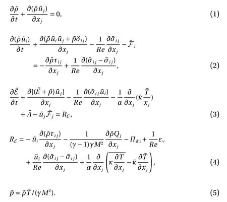
where τijis the SGS stress, Qjis SGS heat flux, Πdilis SGS pressure-dilatation, and ενis SGS viscous dissipation. τijand Qjare the dominant unclosed SGS terms, while other unclosed SGS terms are significantly smaller than the divergence of the SGS heat flux Qjand can be neglected for compressible turbulent flowsinthecurrent Mtand Reλ[37].Inthis paper, the SGS stress τijandtheSGS heatflux Qjare modelled.

The compressible homogeneous isotropic turbulence is numerically simulated by a hybrid compact-weighted essentially non-oscillatory (WENO) scheme in a cubic box of ( 2π)3using a uniform grid with periodic boundary conditions [38]. The hybrid scheme combines an eighth-order compact finite-difference scheme for smooth regions [39] and a seventh-order WENO scheme [40] for shock regions. The force is only applied to the solenoidal component of velocity field by fixing the total kinetic energy in the first two wavenumber shells. Besides, we employ a spatially uniform thermal cooling Λ to sustain the internal energy in a statistically steady state [38].

A fully-connected ANN is used to reconstruct the SGS stress and heat flux as shown in Fig. 1 [21-23]. which consists of four layers (input layer, two hidden layers, and output layer). The neuron numbers of four layers between the set of inputs and finumber of neurons of input layer, while the output layer connal output layer are ( M:1024:512:1), respectively. M is the sists of a single neuron associated with the component of τijand Qj. The transfer function in a layer l is calculated aswhere σ is the activation function,i s the weight, andis the bias parameter.are initialized to uniform by glorot-uniform, andare initialized to zeros. Two hidden layers are activated by a Leaky-Relu activation function:

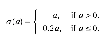
Meanwhile, linear activation σ (a)=a is applied to the output layer. The loss function is defined as 〈(XL-τij)2〉 or〈(XL-Qj)2〉, where 〈〉 represents the spatial average over homogeneous directions (i.e., the entire domain for isotropic turbulence). The back-propagation is used to minimize the loss function.

In this research both the first-order and second-order derivatives of filtered velocity and temperature are used to generate the input variables of ANN. In addition, a thirteen-point stencil is designed to model the effect of spatial structures of flow field at the scales near the filter width Δ. The stencil is determined by the grid length Δg=Δ/2 in each dimension. We consider two sets of input variables:

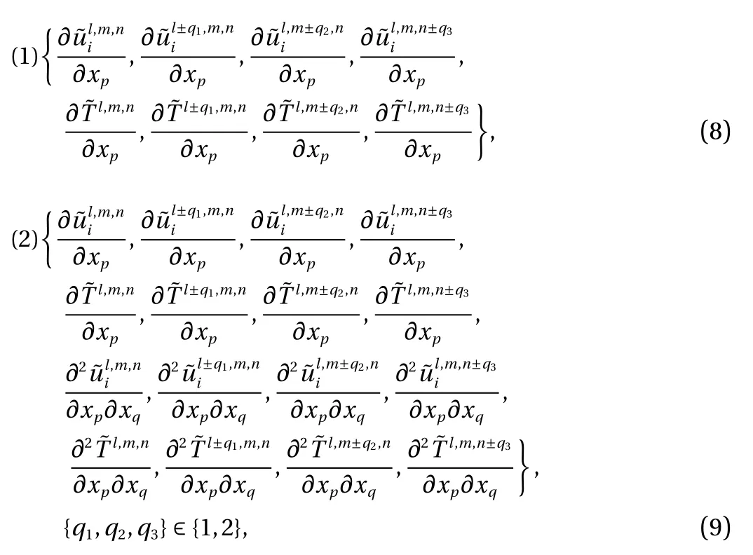
where the indices l, m and n correspond to discrete spatial locationsassociatedwith thegridlength Δg, p,q=1,2,3 arethe subscriptsoftheCartesiancoordinate,and i=1,2,3 isthe subscript of the filtered velocity component. The first set has 156 input neurons M =156, the second set has 624 input neurons M=624. For simplicity, SANN models with the two sets of input variables are abbreviated as SANN-1 and SANN-2, respectively.

In order to increase the robustness of ANN training, all input features XIand output features XOare normalized by, whereandare rms values of the input and output variables. The rms values of SGS terms reconstructed from the gradient model are used in normalizations of output features for ANN training, since the real SGS stress and SGS heat flux are unknown in LES.

LES is performed at grid resolution of 6 43(=Δ/2) with filter width Δ =32Δx . 1 63different data sets of 6 43coarse grid points in three dimensions by using a coarse-graining procedure involves the selection of every sixteenth grid point in each direction in the DNS data. We randomly choose ( 15×64)3grid points for the generation of 7 0% of training data and 3 0% of testing data. Finally, the Adam algorithm is used to train the ANN network [41] for a long duration (1000 epochs), with batch size being 1000 till the learning rate is minimal. The learning rate of the proposed SANN model for 2000 iterations is shown in Fig. 2.The learning process is well-formulated since the training and validation loss are nearly stable after 500 global iterations. It's reasonable to train 1000 iterations of the SANN model.

In an a priori analysis, the performances of the SANN model are evaluated by calculating the correlation coefficient C (H) and the relative error Er(H) of the modeled term Hmodelas compared to the real unclosed SGS term H, where the C (H) and Er(H) are calculated by, respectively,

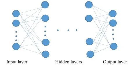
Fig. 1. Schematic diagram of the ANN's network structure.

Meanwhile, two types of gradient models are compared with the SANN models:abbreviatedasVG1m, whereandaredetermined from DNS databyleast square method. Table1 showscorrelation

Thefirstmodel isabbreviatedas VG1. Thesecondmodel is coefficients and relative errors ofτ11,τ12and Q1forthe SANN-1 and SANN-2models inthe testingset.The SANN-1model performs much better than the VG1 and VG1m models. The correlation coefficients are larger than 0.99 for the SANN-1 model,while the VG1 and VG1m models give correlation coefficients about 0.90. The relative error of the SANN-1 model can be less than 8%forτ11,whichismuchsmallerthanthose ofVG1 and VG1mmodels.With morereasonableinput features,theSANN-2 model performs better than other models. Thus, ANN can be used to explore the physical fundamentals of turbulence modeling.

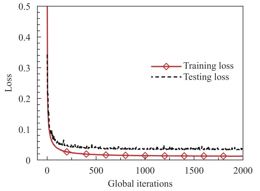
Fig. 2. Learning curve of the SANN-1 model of.

Table 1 Correlation coefficients (C) and relative errors ( ) of, and for different models in the testing set.

Table 1 Correlation coefficients (C) and relative errors ( ) of, and for different models in the testing set.

In order to analyze the impact of spatial stencil sizes of input features, the SANN is trained with the first-order derivatives of filtered velocity and temperature with seven-point stencils({q1,q2,q3}∈{1,2,...,Nq}, Nq=1, M =84), nineteen-point stencils(Nq= 3, M=228) , and twenty-five-point stencils ( Nq= 4,M=300), which are abbreviated as SANN-3, SANN-4 and SANN-5, respectively. The a priori results of the SANN-3, SANN-4, and SANN-5 models are summarized in Table 1. The SANN-1,SANN-4 and SANN-5 models show similar correlation coefficients and relative errors of τ11,τ12,Q1with Nq≥2, indicating that the learning accuracy does not increase significantly with the increase of the size of the stencil for Nq≥2. Though the higher order derivatives have a potential to give higher accuracy, it is difficult to keep numerical stability when considering the third-order derivatives of velocity and temperature as input features.Thus, we have not considered the third order derivatives in this paper. We will focus on the ANN models with optimal stencil size and higher order derivatives in a follow-up study.

In an a posteriroi test, we compare the performance of the SANN-1 model with large eddy simulations without any LES model (No-model), and using the dynamic mixed model (DMM)model [37, 42, 43]. Considering that the differences between LES results and filtered DNS results are mainly due to the LES models for F GR=2, we present a study of the different SGS models at grid resolution of 6 43(hLES=Δ/2, F GR=2) with the filter width Δ=32Δx.

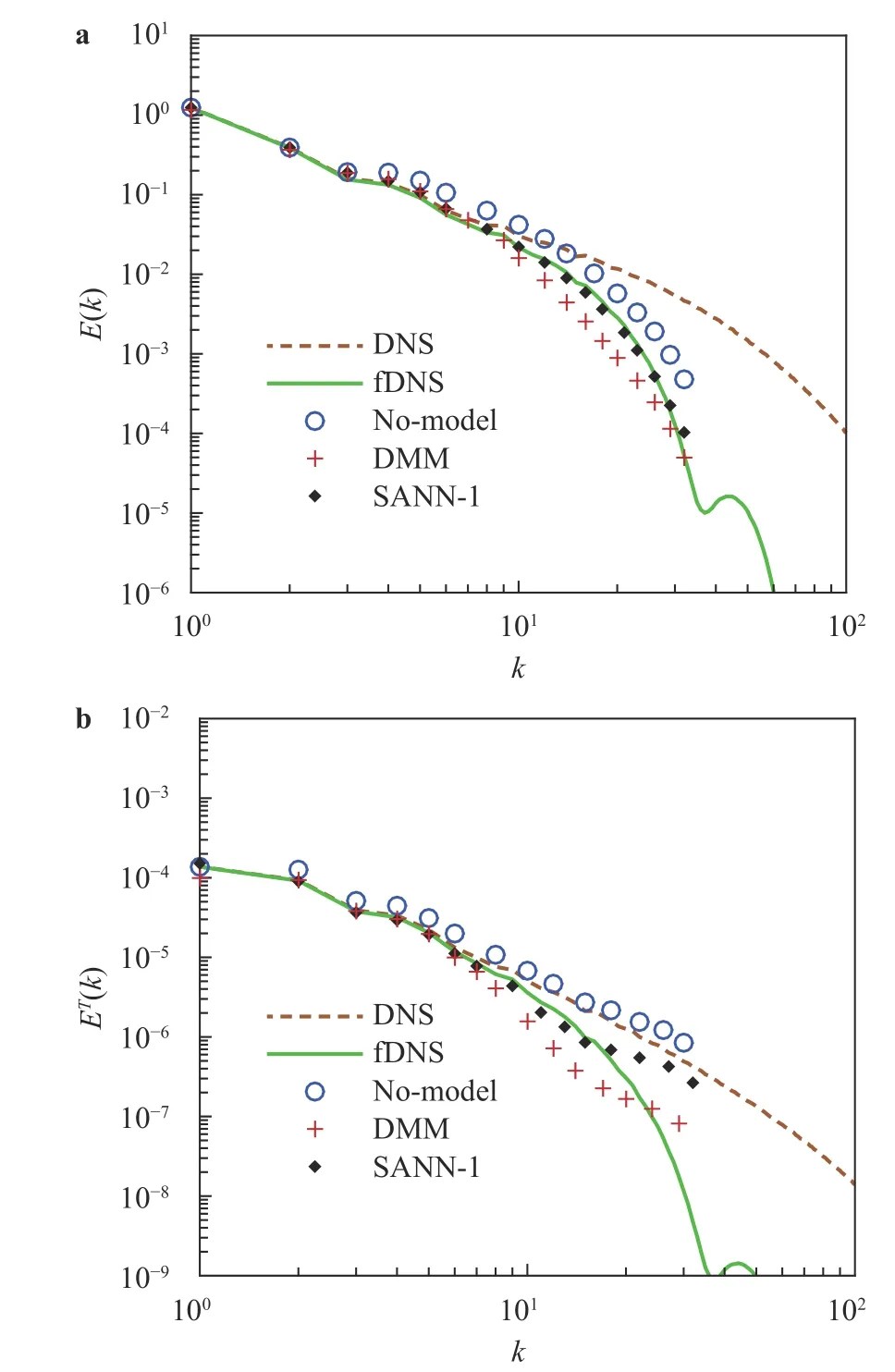
Fig. 3. Spectra of velocity and temperature for LES: a, b.

The spectra of velocity and temperature are displayed in Fig. 3 for the DNS, filtered DNS (fDNS) and LES computations performed with the No-model, DMM and SANN-1 models. There is a long inertial region with a k-5/3scaling of velocity spectrum for DNS results. The errors of the spectra predicted by LES models increase as k increases. The spectrum of the velocity field predicted by the 'No-model' without enough dissipation is higher than that of the fDNS data at large wavenumbers. The spectra of velocity near the cut-off wavenumber are damped too strongly for the DMM model, which show a bumped spectral distribution. The SANN-1 model nearly overlaps with the filtered DNS data without bump for the velocity spectrum. Meanwhile, due to the excessive dissipation near the largest resolved wavenumbers,the temperature spectrum predicted by the DMM model is in reasonable agreement with fDNS for k ≤10 and significantly smaller at large k. Temperature spectrum predicted by the SANN-1 model is almost exactly for wavenumber k ≤20 by catching more smaller thermal scale structures.

Figure 4 shows the probablity density functions (PDFs) of the normalized velocity incrementwhereis the longitudinal increment of the velocity for the separation r . Here rˆ =r/|r|. The velocity increment is normalization by the rms velocity. The PDFs of δrare almost symmetry. The DMM and SANN-1 model can predict the PDFs ofaccurately at large r (r =4Δ) . As r decreases,the SANN-1 model performs better than the DMM model.

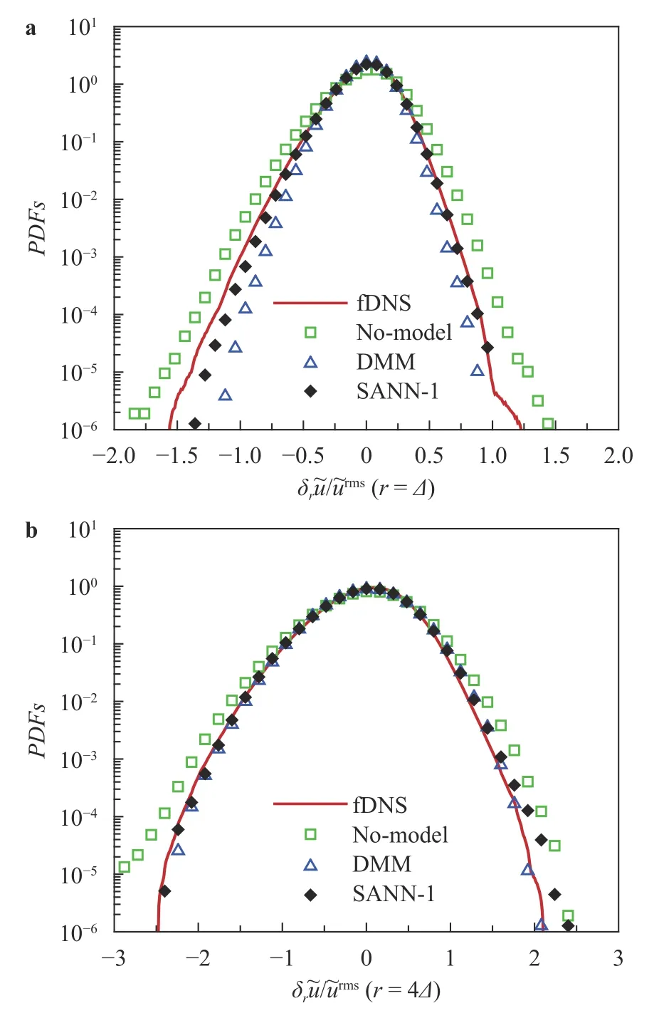
Fig. 4. PDFs of the normalized increments of the velocity for LES.a, b.

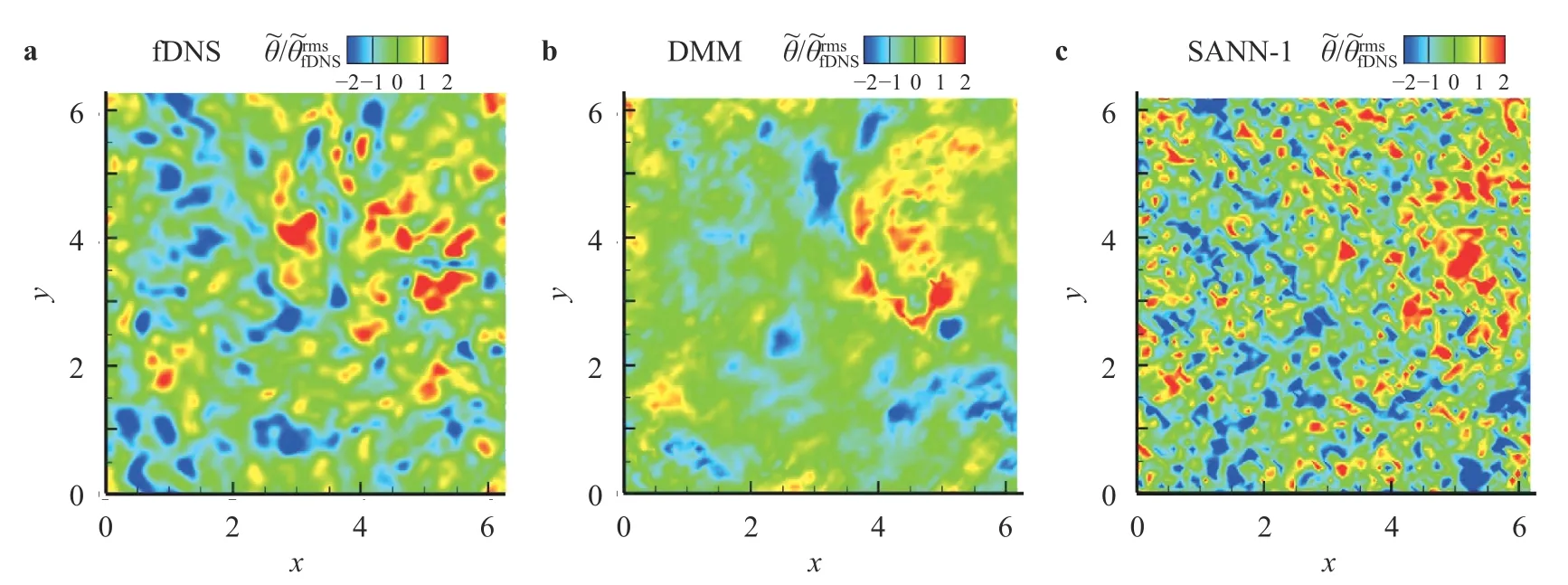
Fig. 5. Contours of the normalized velocity divergence on an arbitrarily selected x-y slice, at (here is the largeeddy turnover time): a fDNS, b DMM, and c SANN-1.

Finally, we compare the instantaneous coherent structures predicted by LES with initial input data from an instantaneous flow field of filtered DNS. The structures of velocity divergence of fDNS and LES with the DMM and SANN-1 models at the same instant are shown in Fig. 5. The large block-like structures of velocity divergence from fDNS can be catched by both DMM and SANN-1 models. The SANN-1 model can recover more smallscale structures than the DMM model.

In this paper, the SGS stress and SGS heat flux of compressible turbulence are reconstructed by using the SANN model with the first and second order derivatives of filtered velocity and filtered temperature at different spatial locations. The SANN models can predict much higher correlation coefficients and much smaller relative errors than the gradient model in an a priori test. In an a posteriori test, the detailed comparisons of the SANN-1 model, No-model and DMM models show: the SANN-1 model performs better than No-model and DMM models in the prediction of spectra and statistical properties of velocity and temperature, and the instantaneous flow structures. In order to develop more advanced SGS models for LES of turbulence, more physical characteristics of SGS unclosed terms should be added to ANN framework, including the nonlinear couplings between velocity and thermodynamic variables, and the spatial-temporal non-locality of SGS dynamics.

Acknowledgements

This work was supported by the National Natural Science Foundation of China (Grants 91952104, 11702127, and 91752201), and the Technology and Innovation Commission of Shenzhen Municipality (Grants KQTD20180411143441009,JCYJ20170412151759222, and ZDSYS201802081843517). This work was also supported by Center for Computational Science and Engineering of Southern University of Science and Technology. J. Wang acknowledges the support from Young Elite Scientist Sponsorship Program by CAST (Grant 2016QNRC001).