Robust control for electric vehicle powertrains

Johannes BUERGER, James ANDERSON

1.BMW Group,Munich,Germany;

2.Department of Computing and Mathematical Sciences,the California Institute of Technology,Pasadena,U.S.A.

Abstract This paper considers the application of robust control methods(μ-and H∞-synthesis)to the speed and acceleration control problem encountered in electric vehicle powertrains. To this end, we consider a two degree of freedom control structure with a reference model. The underlying powertrain model is derived and combined into the corresponding interconnected system required for μ-and H∞-synthesis.The closed-loop performance of the resulting controllers are compared in a detailed simulation analysis that includes nonlinear effects. It is observed that the μ-controller offers performance advantages in particular for the acceleration control problem,but at the price of a high-order controller.

Keywords: Automotive control,electric vehicle powertrains,robust control

1 Introduction

Drivetrain oscillations represent a significant challenge in automotive engineering and consequently this issue has sparked much research interest[1].The main problem arises due to the fact that resonant frequencies of the powertrain are excited either due to changes in the controlled input (i.e., the electric motor torque) or due to external disturbances. These oscillations can lead to uncomfortable longitudinal driving dynamics, since the resonant frequencies of a typical powertrain are in the perceivable range of humans [1]. Furthermore, these oscillations may imply an increased vehicle response time during dynamic driving manoevers,in particular if additional powertrain functions for limiting the electric motor gradient are employed(as is often the case in automotive practice)to reduce the oscillations.Finally,an increased rate of mechanical wear of hardware components may result [2] from excessive oscillations. Compared to drivetrains with combustion engines, electric motors are generally more dynamic than conventional combustion engines.On the one hand,this implies that sharp torque commands will excite the powertrain more severely;and on the other,this implies that electric motors are better suited to damp these oscillations, since their torques can be accurately commanded with very small response times[3].

We consider two particular control problems of fundamental importance to electric vehicle powertrains,the acceleration and speed control problem. In the acceleration control problem the acceleration at the output side of the drivetrain is controlled. This is important in practice for two reasons:First,the driver demand can be interpreted as a demanded torque at the wheel or equivalently as a demanded acceleration at the wheel[4].This implies that the fundamental goal of satisfying the driver demand ultimately has to consider the inherent powertrain dynamics to avoid unnecessary oscillations. Second,in the case of no slip,the rotational acceleration can be related to the longitudinal acceleration of the vehicle.In the speed control problem the speed at the output side of the drivetrain is controlled.This is of importance,since certain powertrain functions can be translated into an equivalent speed demand at the wheels (e.g., if a wheel slip condition is detected, we may command a specific wheel speed to overcome the slip condition).Powertrain oscillation damping for a powertrain with a combustion engine has been addressed as a speed control problem in[3,5,6],in which separate design strategies are employed to obtain a feedback and feedforward controller.Furthermore,robust control ideas have been applied in this context, e.g., in [6] using sliding mode control, or in [3] using H∞-control. Finally, model predictive control has been applied recently in [7], however the realizability of online-optimization based approaches on series-production control units is questionable despite recent advances in numerical optimization techniques.Recent work has addressed this online problem by getting additional help from the cloud [8] and methods for automated embedded code generation for fast operator splitting methods[9]seem promising.

In this paper, we consider a two degree of freedom controller with a reference model,which addresses the preferred approach in automotive practice to consider a pre-stabilization filter with a feedback control loop to minimize feedback control action. Since uncertainty is omnipresent in any powertrain control system, approaches which have explicit robustness properties have proven to be beneficial[3,6].Another important practical advantage is that reference models allow the closedloop system to be shaped by the control designer and also simplify the calibration process. Finally, different driving modes may be translated into specific reference models. While this paper considers the application of H∞and μ-synthesis,we note that alternative robust control methods have been suggested in[10],where a linear parameter-varying controller is developed based on H∞control theory.This is advantageous if knowledge about the variation of system parameters is available. In contrast to this,we also treat system parameters as explicitly uncertain in the design process.In summary,this paper contains two main contributions: First, it considers the acceleration and speed control problem at the output side of the powertrain: we derive a powertrain model which captures the relevant dynamics from an oscillation damping point of view,but is sufficiently compact to allow a robust model-based control design with practical significance.Secondly,for the first time,we apply the two-degree-of-freedom H∞-and μ-synthesis[11,12]to the acceleration and speed control problem in order to minimize the worst case error relative to a given reference model. It is hoped that, in addition to addressing an important applied control problem, that this paper serves as an informative case study in the application of robust control methodologies to automotive applications. In particular, an important practical message is that μ-synthesis can offer substantial benefits, if a high degree of uncertainty is present in the system.

2 System modelling for acceleration and speed control

This section considers the physical modelling for acceleration and speed control at the output side of the powertrain. The schematic of the electric vehicle powertrain model is shown in Fig.1.We consider an electric vehicle where a single axis is propelled by an electric motor. We make the (standard) assumption that the electric motor dynamics are significantly faster than the powertrain dynamics and may therefore be neglected in the control design.The electric motor shaft connects via a single-speed transmission (with a fixed gear ratio g) to the output drive-shaft. The output drive-shaft is connected via a differential to the wheels.It is assumed in common with the literature [1,6] that the dominant part of the powertrain oscillation occurs after the transmission and is characterized by a mass-spring-damper system. We do not consider backlash in the transmission model,however,its effect is separately analysed in the simulation (Section 4). Finally, we consider an additional linearly speed-dependent damping term on the input and output shaft, respectively, e.g., representing viscous friction.

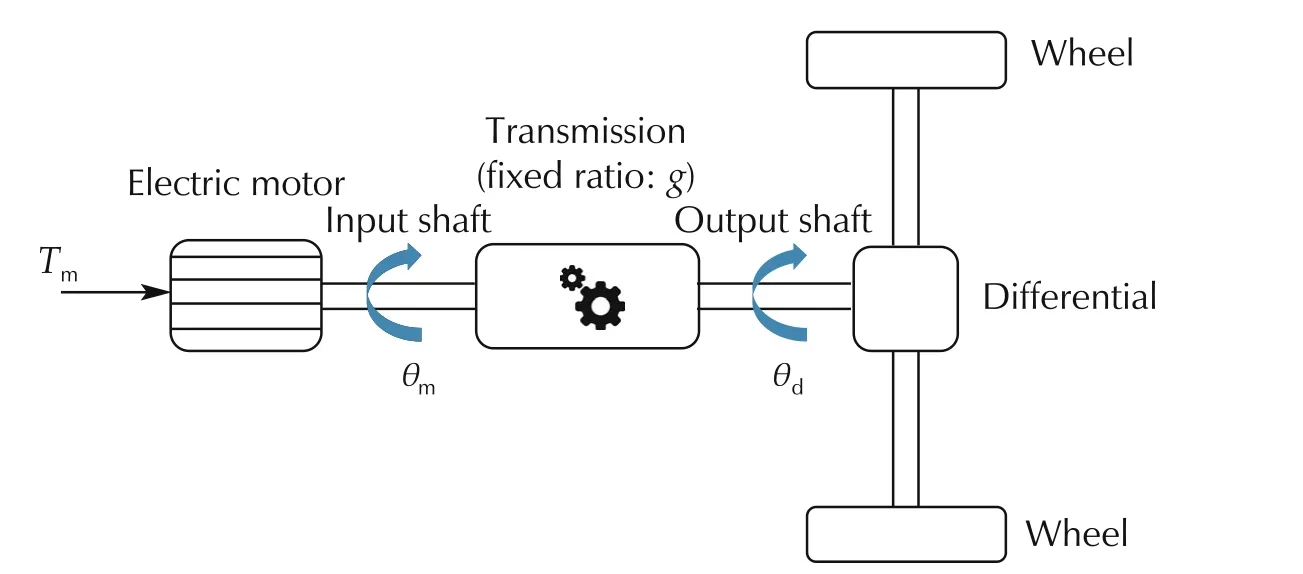
Fig.1 Schematic of the considered electric vehicle powertrain.

Newton’s law is first applied to the input(i.e.,electric motor)shaft to yield

where Jmcorresponds to the combined inertia of the motor and input shaft and θmand θdcorrespond to the angular displacements of the input and output shaft.Tmrefers to the torque generated by the electric motor and can be considered as the system input, k and d denote the inner output shaft elasticity and damping factor and dmdenotes the damping due to the viscous friction of the motor. Newton’s law is then applied again to the output shaft to give

where Jdcorresponds to the combined inertia of differential,shafts,wheels and vehicle mass and ddrefers to the damping at the output side, and k and d are as defined in (1). In the remainder of this section we derive from(1)and(2)state space models of the form:

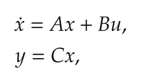
where x,u, and y are the state, input, and output vectors respectively,for the acceleration and speed control problems.

2.1 State-space model for acceleration control

We first consider the case where the controlled output is chosen as the longitudinal acceleration of the vehicle. This is important, since the driver demand can be interpreted as an acceleration command (or torque command at the wheel).Furthermore,this setup allows us to shape the acceleration output according to the desired comfort level via a reference model.

We define the state vector xa,input uaand output yaas

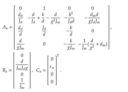
where rwcorresponds to the wheel radius. The input corresponds to the torque delivered by the electric motor and the output to the longitudinal acceleration of the vehicle(for no wheel slip).The corresponding state space matrices(Aa,Ba,Ca)may be obtained from equations(1)and(2)as

2.2 State-space model for speed control

Here,we consider the case where the controlled output is chosen as longitudinal speed.We define the state vector xs,input usand output ysas

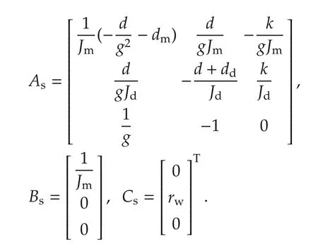
note that the output to the longitudinal speed of the vehicle(for no wheel slip).The corresponding state space matrices(As,Bs,Cs)may be obtained from equations(1)and(2)as

3 Two degree of freedom robust control

In this section, we consider a two degree of freedom control configuration as shown in Fig.2 which is very convenient from a practical point of view, for example, it allows different levels of comfort during tip in/tip out manoevers to be translated directly into a reference model(which may further be configurable by the driver). For simplicity, we choose the reference model to be a second order system. This allows us to translate requirements on the level of comfort and speed of response into an equivalent damping factor and natural frequency.We consider as the controlled output the frequency weighted difference between the actual system output and the reference model output. Our goal is to minimize this difference in a worst case sense using H∞- and μ-control design. A two degree of freedom controller reduces the amount of feedback action,since a pre-stabilization channel is systematically included(which again is convenient from a practical point of view). In this section, we proceed as follows: we first consider the nominal two degree of freedom setup and consider the state-space representation of the associated interconnected system, including parametric uncertainty. This is then related to the corresponding input/output Δ-P-K-structure as shown in Fig.3, which is considered(as standard in the literature,e.g.,[12,13])as the basis for Robust Control Design.The basic steps of H∞-and μ-synthesis are discussed at the end of this section.

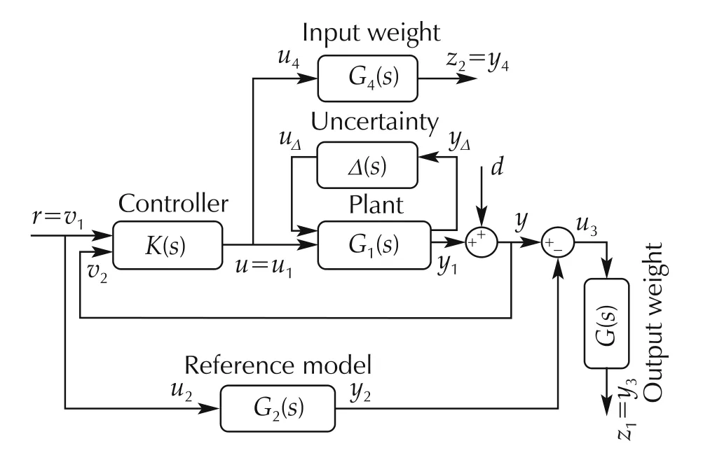
Fig.2 Interconnected system setup for two-degree-of-freedom controller.

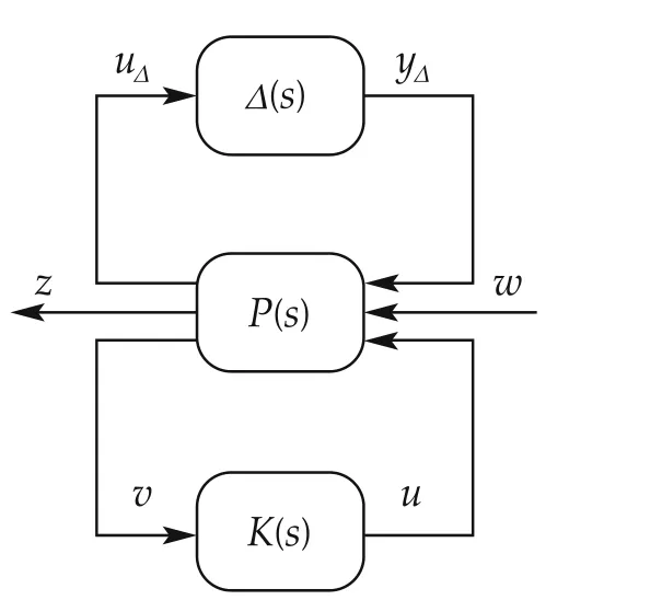
Fig. 3 Input/Output model structure for robust stability and performance.

3.1 Model interconnection

First, we consider the state-space realizations of the plant G1, reference model G2, output weight G3, and input weight G4(c.f.Fig.2)as follows:

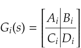
for i=1,...,4.The corresponding state,input and output are denoted by xi∈Rni, yi∈R and ui∈R. From Fig.2,we can relate the input uito Gias1We note here that u is a scalar,and should not be interpreted as a vector containing u1,...,u4.

We continue by defining the external and internal inputs and outputs for the Δ-P-K-structure as follows:

We now consider the state-space representations of Gi(s) together with the chosen interconnection structure. The associated state is given by xic=. Furthermore, we consider uncertainty of the parameters of the powertrain system model. Associated uncertain parameters may be pulled out into the standard form of an uncertain diagonal matrix Δ.The corresponding input and output of Δ is defined as yΔ∈RnyΔand uΔ∈RnuΔ, respectively. As an example we consider uncertainty in the output shaft elasticity k and consider the third row of the matrix Aa: The particular parameter may be expressed as kδ=k(1+pkδk).We find the associated ith diagonal entry of Δ by consideringandwhere pkis the percentage of the parameter uncertainty of k and δk∈[-1,1].As shown in Fig.3,we consider the collection of inputs and outputs as uic= [,w1,w2,u]Tand yic=[,z1,z2,v1,v2]T,respectively.Overall we obtain the following state space open-loop system description by using the conditions(3):

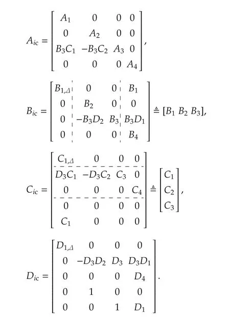
The corresponding transfer function matrix P(s)of the Δ-P-K-structure is then obtained by recalling the definition of the inputs w,u of(4)and of the outputs z,v of(5),so that using uic=[wTuT]Tand yic=[zTvT]Twe can relate the input to the output by the relation yic(s)=P(s)uic(s)with

3.2 Weighting functions

The weighting functions G3and G4required for the robust control design of Section 3 are chosen as

for the output and input respectively(see Fig.2)in both the acceleration and speed control context. The choice of first-order lead-lag type weight functions allows us to penalize output deviations relative to the reference model in the lower frequency range up to above the resonance frequencies (20-50 rad/s as depicted in Fig.4),while the magnitude decreases thereafter for higher frequencies above resonance (see Fig.5), by selecting the relevant time constants of the corresponding weight transfer functions.Similarly,the input weight is designed to be flat up to above the resonant frequency and increases thereafter to avoid unnecessary control action in the high frequency range(see Fig.6).The scalings of the weight functions can be seen as calibration parameters and are used to trade off performance requirements(tracking) and constraint satisfaction requirements on the inputs. We note that the weight functions are chosen identical for the H∞and μ-controllers.

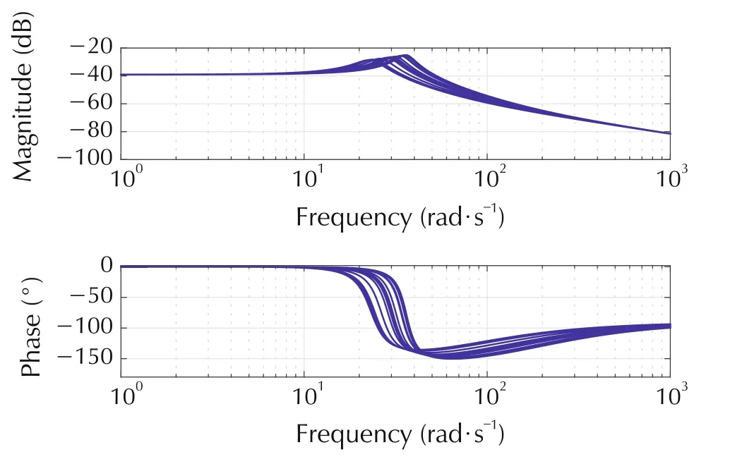
Fig.4 Open loop(i.e.,u1 to y1 in Fig.2 with no controller)Bode plot for acceleration control with uncertain shaft elasticity k,we allow for nominal±50%deviation.

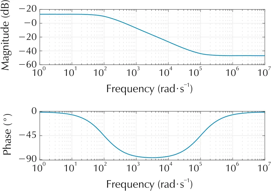
Fig.5 Weighted output G3 Bode plot.

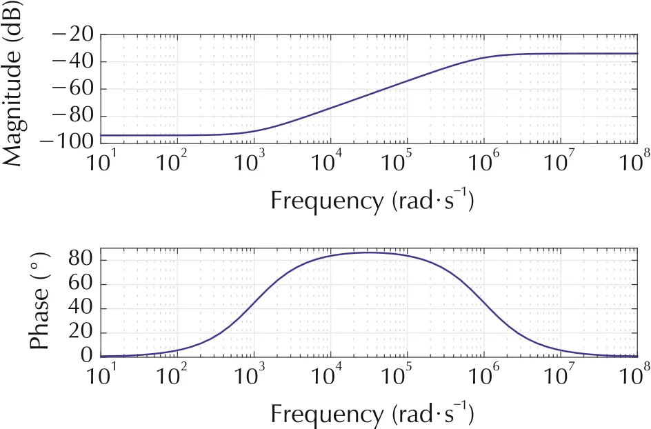
Fig.6 Weighted input G4 Bode plot.

3.3 Controllers

For H∞-design we consider the reduced setup without parametric uncertainty and define the associated transfer function matrix:

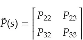
with inputs w and u and outputs z and v.By considering the lower fractional transform(see[13]):

we can relate the external input w to the external output z by z=Fl(,K)w.We note that the entries of the transfer function matrix Flmay be interpreted as follows:The element relating w2= d to z2= y4is the weighted output sensitivity due to a disturbance, w1= r to z2= y4corresponds to the transfer function from reference input to the weighted error between reference model and actual output. The transfer function w2= d to z1= y3is the weighted control action due to a disturbance and w1= r to z1= y3corresponds to the weighted control action due to the reference input. In order for the control problem to make sense,we have that(A,B3)is stabilizable,and(C3,A)is detectable.

To find the optimal H∞-controller KH∞(s)we need to solve the following minimization problem:

and its solution may be obtained using an iterative procedure by solving a sequence of two coupled algebraic Riccati equations for associated suboptimal values of γ ≥γopt,where γopt=‖Fl(KH∞)‖∞(c.f.[13]).

We are now ready to analyse robust stability and robust performance: First we construct the lower fractional transform N = Fl(P,K) (i.e., the feedback interconnection of the plant and the controller). Using N we incorporate the uncertainty block Δ by forming the upper fractional transform F = Fu(N,Δ) =N22+ N21Δ(I - N11Δ)-1N12. Note that F defines the mapping between the external input w and output z.We note that in this paper we are interested in parametric uncertainty which,as illustrated in Section 3.1,leads to a diagonal matrix Δ.In general,the set of admissible perturbations may be defined as

where Δ is a block diagonal matrix representing uncertain perturbations on the system. Robust stability requires that F is stable for all allowable Δ ∈Δ or,equivalently,the structured singular value μΔ(N11)＜1 for all frequencies ω and stable N2The structured singular value is defined as μΔ(N):=(inf{¯σ(Δ)| det(I-NΔ)=0,Δ ∈Δ})-1.For more details on μ the reader is referred to[14].. Robust performance requires‖F‖∞≤1 for all allowable Δ ∈Δ or,equivalently,the structured singular valuefor all frequencies ω whereis the block diagonal matrix of Δ and an additional fictitious performance uncertainty block Δp,i.e.,=diag{Δ,Δp}[14].

On the other hand, for comparison, we consider a controller based on μ-synthesis, i.e., a controller design directly based on minimizing the structured singular value, so that by design robust stability and performance can be guaranteed(see[12,13]):

In practice, methods based on the so-called D-K iteration provide a computationally feasible approach to obtain an approximate solution.This method considers an upper bound onusing diagonal scaling matrices(i.e.,where D is defined as the set of matrices that commute with).The procedure consists of two steps at each iteration:an H∞-optimization-step and an D-scaling optimization step.

Finally, we note that the resulting controllers contain two transfer functions in our application in both the H∞-and μ-synthesis context,i.e.,K(s)=[Kv1(s) Kv2(s)].This controller may be translated into a classical feedforward/feedback structure (with reference input r and feedback error signal e = r- y) by setting u = Kv1r+Kv2y=(Kv1+Kv2)r-Kv2(r-y).

4 Simulation

This section considers the application of the robust control algorithms of Section 3 to the electric vehicle model for speed and acceleration control developed in Section 2. The parameters chosen are listed in Table 1 and the open-loop step response is shown in Fig.4.

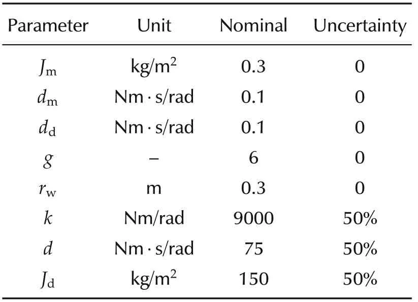
Table 1 Nominal parameter values and their respective uncertainty ranges.

We consider uncertainty in the parameters describing inner output shaft elasticity, damping factor, and combined inertia, k,d,Jdrespectively. Intuitively, Jdtakes into account the uncertainty in a vehicles’s mass, e.g.,fuel load,number of passengers,etc.A sensitivity analysis reveals that the parameter k has the strongest negative impact on the system and is taken as the only explicitly uncertain parameter against which the μ-controller is designed.Thereby we follow the rule of thumb in robust control that in order to limit the complexity(the order)of the controller only the essential uncertain information should be included - this will become apparent in the the following sections. From a practical standpoint the uncertainty is chosen relatively large to demonstrate the effectiveness of the μ-based controller. In practice,the uncertainty may be lower and to allow the reader to evaluate the resulting effects,we have included step responses with reduced levels of uncertainty in Fig.7.

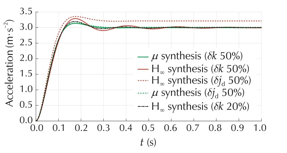
Fig.7 Worst case closed-loop response of μ-and H∞acceleration controller for uncertain shaft elasticity k and load inertia Jd.

4.1 Acceleration control

We choose the reference model as a second order system with natural frequency ω0= 25 rad/s and damping factor ζ=0.7.This corresonds to a relatively good compromise between sportiness and comport due to the chosen damping factor. The chosen natural frequency affects the speed of response,but also has to be chosen so that in the operating range of the system the actuator constraints are not violated (±600 Nm). In general, the actuator constraints can be addressed by considering a step input from zero to the maximum acceleration for a given choice of the reference model and input/output weight functions. If this leads to actuator constraint violations, either the weight functions can be scaled or the reference model dynamics can be reduced. The μcontroller synthesis using DK-iterations(performed using[15])converges to a controller satisfying robust performance and stability as shown in Fig.8 with a corresponding minimal value of γ = 6.48. The design leads to a controller order of 80 and a resulting closed-loop system order of 88.The closed-loop Bode plot is shown in Fig.9,which shows a relatively narrow spread of the family of frequency responses over k. A nominal response of the controller and the corresponding input trajectory (the motor torque) is shown in Fig.10. This input trajectory shows the characteristic dip necessary to avoid exiciting the resonant frequency.By considering the worst case step response in Fig.7,we can conclude that we obtain a good tracking behaviour of the reference model.For an uncertain inertia Jd(against we have not designed the μ-controller)one can further conclude that the controller is robust and leads to a very small steady state error.

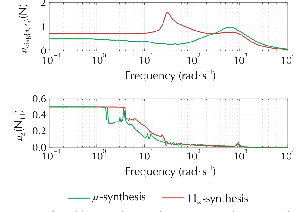
Fig. 8 Closed-loop μ for acceleration control. Top: Performance.Bottom:Stability.

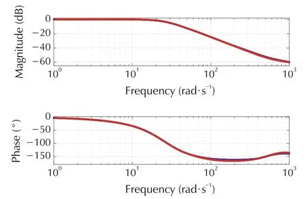
Fig.9 Closed-loop Bode plot for μ acceleration controller for uncertain shaft elasticity k.

The H∞-controller synthesis (performed using [15])converges to a minimal value of γ = 6.37 with a controller order 8 and resulting closed-loop system order of 16.This is due to the fact that the weighting functions G3and G4are both first order systems, and the reference model G2is second order, thus the total plant order is 8.The closed-loop Bode plot is shown in Fig.11,which shows a relatively wide spread of the family of frequency responses over k in the 11-13 rad/s range.By considering the worst case step response in Fig.7, we can conclude that in this case the resonance frequency is excited and leads to an unpleasant oscillatory response. Fig.8 furthermore tells us that we do not get robust performance as in the top plot μ ＞1.Finally,for an uncertain inertia Jd, one can further conclude that this leads to a significant steady-state offset.

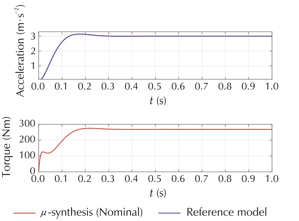
Fig.10 Nominal closed-loop response of μ acceleration controller and input trajectory Tm(t).

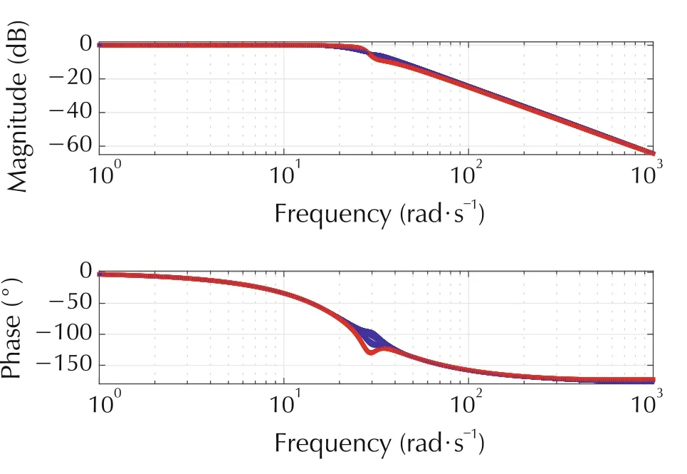
Fig. 11 Closed-loop (i.e., r to y in Fig.2) Bode plot for H∞acceleration controller with uncertain shaft elasticity k.

Finally the synthesized controllers are used in a simulation model including the digital implementation of the controllers and by considering nonlinear characteristics such as backlash. The simulation considers a digital implementation of the robust controller with a sampling rate of 1ms(by conversion of the corresponding controller transfer functions to discrete time). This process can lead to numerical difficulties for the high order μ controller. This is overcome by reducing the model order to 25 using Hankel singular value based model order reduction. With respect to backlash, we note that in practice often additional powertrain functions may be used(not considered in this paper),which detect backlash and consequently limit the gradients of the requested torque and therefore allow the problem to be reduced [16]. We consider backlash in the transmission between the input and output shaft(Fig.1)and use a backlash dead zone model detailed in[16]with a backlash angle of 20°. The results in Fig.12 show that both controllers request large control actions in order to track the reference model.We note that the μ-controller performs significantly better in this situation with only a small, temporary deviation from the reference, while the H∞-controller leads to an oscillatory response.

Overall we conclude that the μ-controller significantly outperforms the H∞-controller in the presence of parameter uncertainty or backlash, but at the price of a considerable increase in the complexity of the controller.Also we note from Fig.12 that the μ controller is more aggressive and requires ±500 to gain its performance(which is however within the actuator constraints considered).

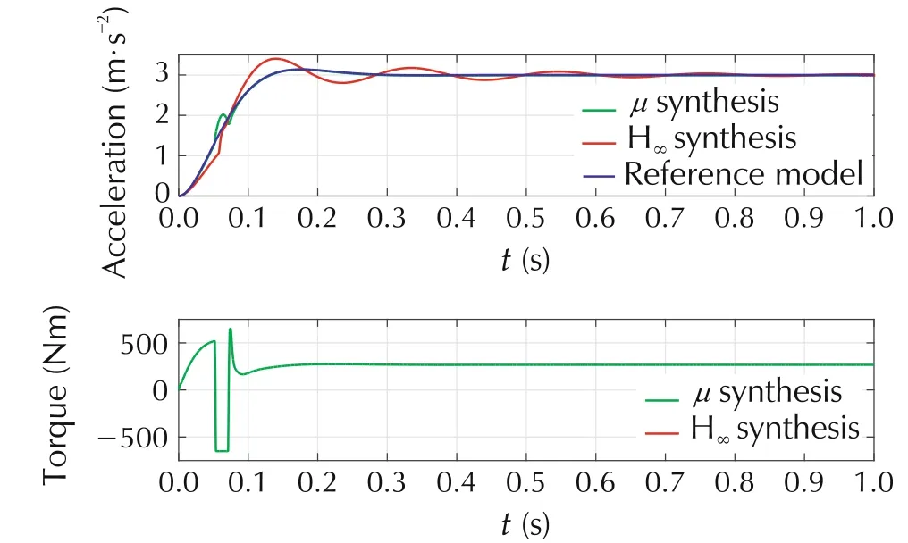
Fig.12 Closed-loop response of μ-and H∞acceleration controller in the presence of backlash.

4.2 Speed control

This section considers the speed control problem and the open-loop Bode plot is shown in Fig.13.We consider the same weighting functions as for the acceleration control problem,but employ a slower second order system with a natural frequency of ω0= 2 rad/s and damping factor of ζ = 0.7 as a reference model, since otherwise very large(and unrealizable)inputs would result.

The μ-controller synthesis using DK-iterations (performed using [15]) again converges to a controller satisfying robust performance and stability as shown in Fig.14 with a corresponding minimal value of γ=0.87.The design leads to a controller order of 9.The closedloop Bode plot is shown in Fig.15, which shows a relatively narrow spread of the family of frequency responses over k and a dip in the magnitude plot at around the resonant frequency of the system.

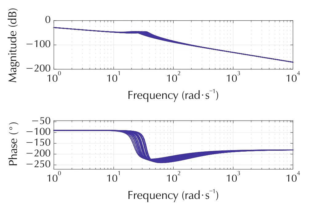
Fig. 13 Open loop Bode plot for speed control for uncertain shaft elasticity k.

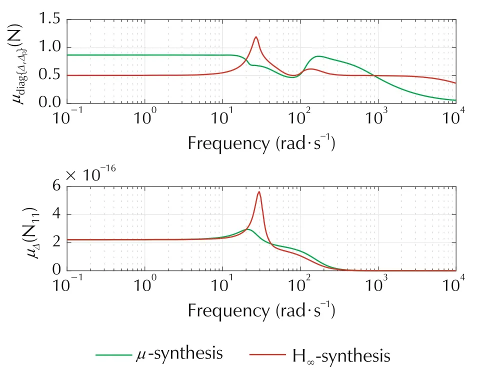
Fig. 14 Closed loop μ for speed control. Top: Performance.Bottom:Stability.

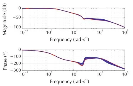
Fig. 15 Closed-loop Bode plot for μ speed controller for uncertain shaft elasticity k.

The H∞-controller synthesis converges to a minimal value of γ = 0.5 with a controller order 7. The closedloop Bode plot is shown in Fig.16,which shows a small increase in the frequency response magnitude plot near the resonant frequency.

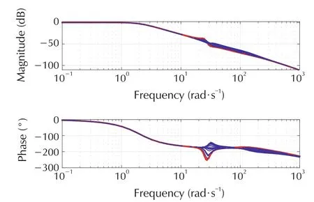
Fig. 16 Closed-loop Bode plot for H∞speed controller for uncertain shaft elasticity k.

By considering the worst case step response in Fig.17,we can conclude that we obtain a good tracking behaviour of the reference model for both μ- and H∞-controllers,despite the fact that the H∞-controller cannot guarantee robust performance as shown in Fig.14.There is only a slight performance advantage of the μcontroller in the initial tracking phase(see Fig.18).

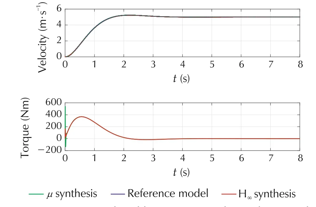
Fig.17 Worst case closed-loop response of μ-and H∞acceleration controller for uncertain shaft elasticity k.

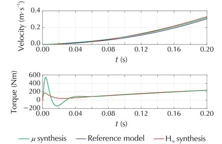
Fig. 18 Worst case closed-loop response of μ- and H∞acceleration controller for uncertain shaft elasticity k - detail of initial phase.

Overall, however we conclude that there are only minimal performance differences between μ- and H∞-control for the speed control problem.

5 Conclusions

This paper has presented a comparative approach to the powertrain control of an electric vehicle based on robust control techniques for a two degree of freedom setup, which is very convenient from a practical (calibration) point of view. The paper has derived the relevant system models required for robust control design.Finally in an extended simulation study it has been demonstrated that the μ-controller offers significant advantages in the presence of uncertainty for the acceleration control problem, however at the price of a high order controller.However,in the speed control setting,the μ controller outperforms the H∞controller with only a two state increase in controller complexity.Future extensions may consider robust model predictive control applications as another interesting comparison for the methods considered in this paper.