Adaptive dynamic programming for finite-horizon optimal control of linear time-varying discrete-time systems

Bo PANG ,Tao BIAN ,Zhong-Ping JIANG

1.Control and Networks(CAN)Lab,Department of Electrical and Computer Engineering,Tandon School of Engineering,New York University,Brooklyn,NY 11201,U.S.A.

2.Bank of America Merrill Lynch,One Bryant Park,New York,NY 10036,U.S.A.

Received 15 August 2018;revised 24 October 2018;accepted 26 October 2018

Abstract This paper studies data-driven learning-based methods for the finite-horizon optimal control of linear time-varying discretetime systems.First,a novel finite-horizon Policy Iteration(PI)method for linear time-varying discrete-time systems is presented.Its connections with existing infinite-horizon PI methods are discussed.Then,both data-driven off-policy PI and Value Iteration(VI)algorithms are derived to find approximate optimal controllers when the system dynamics is completely unknown.Under mild conditions,the proposed data-driven off-policy algorithms converge to the optimal solution.Finally,the effectiveness and feasibility of the developed methods are validated by a practical example of spacecraft attitude control.

Keywords:Optimal control,time-varying system,adaptive dynamic programming,policy iteration(PI),value iteration(VI)

1 Introduction

Bellman’s dynamic programming(DP)[1]has been successful in solving sequential decision making problems arising from areas ranging from engineering to economics.Despite a powerful theoretical tool in optimal control of dynamical systems[2,3],besides the wellknown “Curse ofDimensionality”,the originalDP isalso haunted by the “Curse of Modeling”[4],i.e.,the exact knowledge of the dynamical process under consideration is required.Reinforcement learning(RL)[5,6]and adaptive dynamic programing(ADP)[7-12]are promising to deal with this problem.RL and ADP find approximate optimal laws by iteratively utilizing the data collected from the interactions between the controller and the plant,so that an explicit plant model is not needed.Over the past decade,many papers have been devoted to this routine,for systems characterized by linear or nonlinear,differentialordifference equations.Forexample,adaptive optimal controllers were proposed without the knowledge of system dynamics,by using policy iteration(PI)[7,8,13-15]or value iteration(VI)[16,17],and many references therein.

However,most existing results focus only on the infinite-horizon optimal control problem for timeinvariantsystems.There are relatively few studies on the finite-horizon optimal control problem for time-varying systems.Although finite-horizon approximate optimal controllers were derived for linear systems in[18,19],and nonlinear systems in[20-24],the authors of these papers assumed either the full knowledge of system dynamics,or time-invariant system parameters.Recently,several methods that do not require the exact knowledge of system dynamics have also been proposed for the finite-horizon control of time-varying systems.Extremum seeking techniques were applied to find approximate finite-horizon optimal open-loop control sequences for linear time-varying discrete-time(LTVDT)systems in[25,26].A dual-loop iteration algorithm was devised to obtain approximate optimal control for linear time-varying continuous-time(LTVCT)systems in[27].Different from the time-invariant and infinite-horizon case where the optimal controller is stationary,in the time-varying and finite-horizon case the optimal controller is nonstationary.This brings new challenges to the design ofdata-driven,non-modelbased optimalcontrollers when the precise information of time-varying system dynamics is not available.

This paper considers the finite-horizon optimal control problem without the knowledge of system dynamics for LTVDT systems.Firstly,a novel finite-horizon PI method for LTVDT systems is presented.On one hand,the proposed finite-horizon PI method can be seen as the counterpart to the existing infinite-horizon PI methods,which may be found in[28]for LTVDT systems,in[29]for LTVCT systems,in[30]for linear timeinvariant discrete-time(LTIDT)systems,and in[31]for linear time-invariant continuous-time(LTICT)systems,respectively.On the other hand,it is parallel to the finite-horizon PI for LTVCT systems in[32](Theorem 8).Secondly,we prove that in the time-invariant case,as the time horizon goes to infinity,the finite-horizon PI method reduces to the infinite-horizon PI method for LTIDT systems.Thirdly,we propose data-driven offpolicy finite-horizon PI and VI algorithms to find approximate optimal controllers when the system dynamics is unknown.The proposed data-driven algorithms are offpolicy,by contrast,the methods in[25-27]were onpolicy.In addition,the work[25-27]only considered special cases of linear systems or lacked convergence analysis.Finally,we simulate the proposed methods on a practical example of spacecraft attitude control with time-varying dynamics.The simulation results demonstrate the effectiveness and feasibility of our data-driven finite-horizon PI and VI algorithms.

The restofthispaperisorganized asfollows:Section 2 introduces the problem formulation and necessary preliminaries;Section 3 first presents the finite-horizon PI method,and then its connections with infinite-horizon PI method under certain conditions are revealed;Section 4 derives the data-driven finite-horizon PI and VI algorithms;in Section 5,the application of the proposed methods to spacecraft attitude control is provided;Section 6 concludes the whole paper.

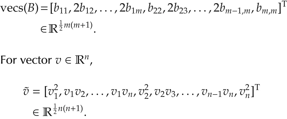
Notations Throughoutthis paper,R denotes the set of real numbers,Z+denotes the set of nonnegative integers.k∈Z+denotes the discrete time instance.X(k)is denoted as Xkfor short and the time index is always the first subscript if it has multiple subscripts,e.g.,Xk,i1,i2.⊗is the Kronecker product operator.For matrix A ∈ Rn×m,vec(A)=,where aiis the i th column of A.For symmetric matrix B ∈ Rm×m,

|·|is the Euclidean norm for vectors and ‖·‖represents the induced matrix norm for matrices.

2 Problem formulation and preliminaries

Consider the following linear time-varying discretetime system:

where k∈[k0,N)is the discrete time instant,xk∈Rnis the system state,uk∈ Rmisthe controlinput,Ak∈ Rn×nand Bk∈ Rn×mare time-dependent system matrices.

We are interested in finding a sequence of control inputsto minimize the following cost function with penalty on the final state

where Qj∈ Rn×n,Rj∈ Rm×m,F ∈ Rn×nare symmetric weighting matrices satisfying Qj?0,Rj＞0,and F?0.

When the system matrices Akand Bkare precisely known for all k∈[k0,N),this is the well-known finitehorizon linear quadratic regulator(LQR)problem(see[2,Pages 110-112]).The optimal control input is given by

and the optimal cost is given by

with the symmetric and positive semidefinite matricesthe solutions to the discrete-time Riccati equation

with the terminal condition=F.Obviously,given a fixed matrix F,the matrix seriesare uniquely determined.

Remark 1 Note that(5)shares similar features with the VI for infinite-horizon discrete-time LQR problem[33,Theorem 17.5.3].In Section 4.2,we will develop a VI-based finite-horizon ADP based on(5).

Remark 2 For the optimal control problem considered here,the optimalcontrol u＊always exists,no matter whether system(1)is controllable,stabilizable or not.This fact can be verified by a straightforward application of DP to system(1)and cost function(2)(see[2,Pages 110-112]).

When Akand Bkare unknown,due to the difference between(5)and the algebraic Riccati equation(ARE)in infinite-horizon control problems(see[2,Page 113]),existing infinite-horizon data-driven methods(see,e.g.,[34,35])cannot be used here directly.Moreover,the methods in[25]and[26]are on-policy and only applied to linear systems with scalar input.By exploiting the property of the cost function,new off-policy methods that find the optimal control inputs without the knowledge of system matrices can be derived.

Now,applying a sequence u(L)of control inputs uk=-Lkxk,k∈[k0,N)with arbitrary gain matricesto system(1),we have

Then the cost at time instance k,k∈[k0,N],can be rewritten as

By using(7)with k1=k+1,k2=k and(9),the following Lyapunov equation can be obtained:

3 Finite-horizon policy iteration for linear time-varying discrete-time systems

For convenience,next,we use A(i)kto denote the closed-loop system matrix at time instance k in i th iteration,i.e.,

3.1 Finite-horizon PI for LTVDT systems

Theorem 1 For system(1),consider the finitehorizon linear quadratic regulator problem with respect to the cost function(2).

1)Choose arbitrary initial gain matrices,and let i=0.

2)(Policy evaluation)Solve for0,by using the following Lyapunov equations with

3)(Policy improvement)Solve for,by using the following equations:

4)Let i=i+1,and go to Step 2).Then for all k∈[k0,N],it holds:

Proof i)Note that

Substituting the above equations into(12)gives

Note that,by(13),there is

Thus,the last two terms in expression(14)vanish.Then we have

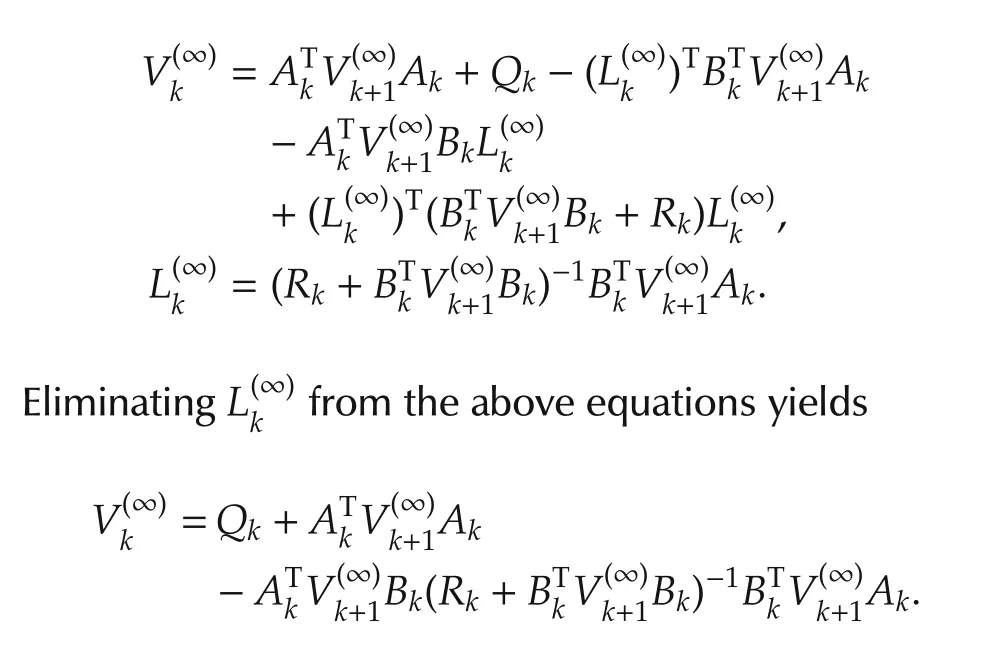
This is exactly the Riccati equation.Due toF and the uniqueness of solution to Riccati equation,follows.This completes the proof.

Remark 3 Most existing numerical finite-horizon optimal control methods were developed for continuous-time models;see[18,22,23],to name a few.It is not clear how to adapt their model-based methods into data-driven algorithms.On the basis of Theorem 1,one can derive corresponding data-driven off-policy PI algorithm(see Section 4).

3.2 Connections with infinite-horizon PI

In this section,we investigate properties of the finitehorizon PI in Theorem 1 as the final time N→ ∞.It is shown that,as N→∞,the proposed finite-horizon PI reduces to the infinite-horizon PI,i.e.,Hewer’s algorithm proposed in[30].

Assumption 1 Throughout this section,we assume stationary system(A,B)and constant matrices Q?0,R＞0,F=0.In addition,(A,B)is controllable,and(A,Q1/2)is observable.

For convenient reference,the infinite-horizon PI algorithm is summarized in the following lemma.

Lemma 1 If staring with an initial stabilizing control u(0)=-L(0)x,setting i=0,the following three steps are iterated infinitely:

1)(Policy evaluation)Solve for V(i)from

where A(i)=A-BL(i).

2)(Policy improvement)Obtain improved control gain

3)Let i=i+1,and go to 1).Then,

i)V(i)?V(i+1)?P＊,∀i∈ Z+.

and the corresponding stationary optimal control u＊=-L＊x,where

minimizes the infinite-horizon cost function

iii)A(i)is a Schur matrix for each i∈Z+.V(i)is the unique positive definite solution to Lyapunov equation(16),and the cost under control u(i)=-L(i)x is given by

In the rest of this section,let thenote the solutions to equations(12)and(13),respectively;(V(i),L(i))denote solutions to equations(16)and(17),respectively;)denote the solutions to equations(5)and(4),respectively;(P＊,L＊)denote solutions to equations(18)and(19),respectively.Note that for fixed=F and free,N→∞implies k→-∞.

Theorem 2 In stationary case,if initial control gains are chosen as,for all k∈[k0,N)in Theorem 1,where L(0)is the same with that in Lemma 1,and F=0,then,as N→∞.Thus,as N goesto the infinity,the finite-horizon PIin Theorem 1 reduces to the infinite-horizon PI in Lemma 1.

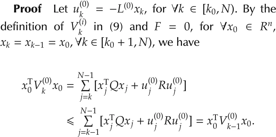
Note that the above inequality holds for all x0∈Rn,thus we know thatis a nondecreasing sequence.Furthermore,for every k?N-1,is bounded from above by the costSince for the same initial conditional x0and same stabilizing controlis equal to the sum of only first N-k terms in equation(21).Thus as k→ -∞,is a nondecreasing sequence and bounded from above by V(0).Again,by the theorem on the convergence of a monotone sequence of self-adjoint operators(See[36,Pages 189-190]),exists.Since A,Q and R are time invariant,letting k→ -∞in(12),we have

Obviously,this is the same form with Lyapunov equation(16).Due to the uniqueness of the solution to Lyapunov equation(16).We knowThis means in the limiting case,policy evaluation step(12)and policy improvementstep(13)in Theorem 1 reduce to(16)and(17)when i=0,respectively.By induction,hold for all i＞0.This proves that,in the limiting case N→∞,the proposed finite-horizon PI in Theorem 1 reduces to the Hewer’s algorithm,i.e.,Lemma 1.This completes the proof.

Remark 4 There are two iteration variables in Theorem 1:time index k and algorithmic iteration index i.The relationships between different value-control pairs with respect to these two iteration variables are summarized in Fig.1.The convergence ofas k→ -∞is proved in Theorem 2;the convergencethe convergence of(V(i),L(i))to(P＊,L＊)is the Hewer’s algorithm[30];the proof of convergence of(P＊,L＊)can be found in[2,Proposition 3.1.1].is the main result in Theorem 1;

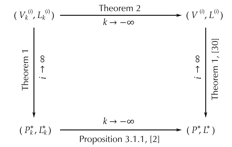
Fig.1 Value-control pair relationships of policy iteration.

Remark 5 When system(1)is periodic,it is also true that the proposed finite-horizon PI reduces to the infinite-horizon PI for periodic systems as N→∞.The infinite-horizon PI for discrete-time periodic linear systems can be found in[37](Theorem 3).In[38](Theorem 3.1),it was shown that,the optimal control problem of discrete-time periodic linear system can be transformed into an equivalent optimal control problem of linear time-invariant system.Thus it is straightforward to extend Theorem 2 to periodic systems.

Remark 6 It is easy to see from[14]that in stationary case,(5)reduces to the infinite-horizon discrete-time VI,by definingin[33,Theorem 17.5.3].

4 Adaptive optimal controller design for linear time-varying discrete-time systems

This section applies adaptive dynamic programming to derive novel data-driven algorithms without precise knowledge of the system dynamics based on Theorem 1 and equation(5),respectively.

4.1 PI-based off-policy ADP

Suppose that a series of control inputs{u(0)

k}N-1k=k0is applied to the system to generate data,and we are in the i th stage of the procedure in Theorem 1.Then(1)can be rewritten as Substituting(12)into equation(23)and rearranging the terms,we obtain

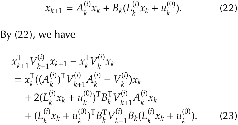
Using the properties of Kronecker product,

where a∈Rn,b∈Rm,W ∈Rn×m,A,B,C,D are matrices with compatible dimensions,the equation(24)can be rewritten as

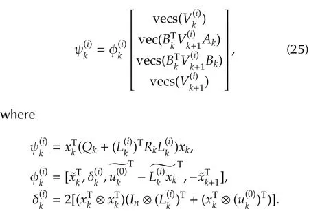
For fixed k,(25)is a degenerate linear equation,since there is only one data triad(,yet at leastunknown variables to solve.Therefore,more data needs to be collected.To this end,suppose in total l groups of different control sequences,j=1,2,...,l are applied to the system and corresponding data is recorded.Each group of control sequences can choose the following form:

where wk,j∈Rmis the exploration noise used to achieve sufficient excitation of the system.By defining the following data matrices:

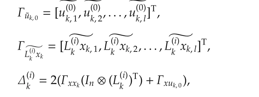
we obtain the matrix equation

where

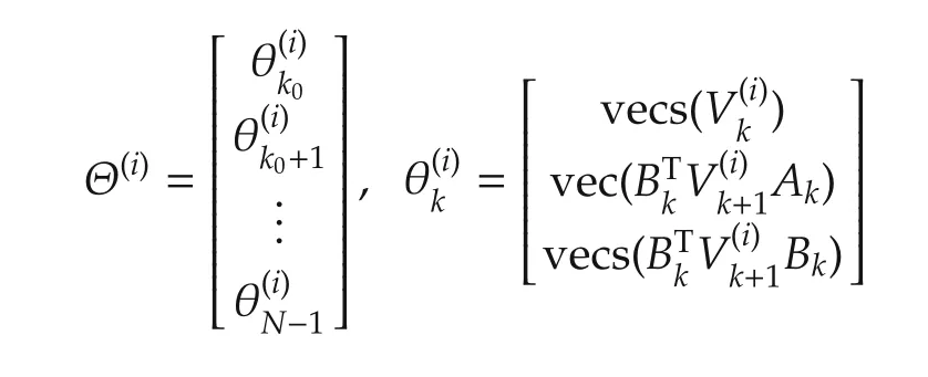
and Ψ(i),Φ(i)are given in(28)and(29)below.

If Φ(i)is a full-column rank matrix,(27)can be uniquely solved,i.e.,

Now we are in the place to present the data-driven off-policy policy iteration algorithm.

Next,the convergence analysis of Algorithm 1 is presented.

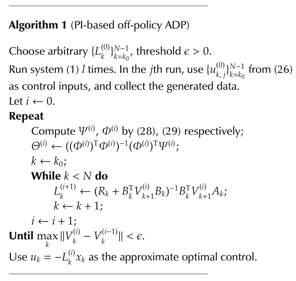
Algorithm 1(PI-based off-policy ADP)Choose arbitrary{L(0)k}N-1 k=k0,threshold ϵ＞ 0.Run system(1)l times.In the j th run,use{u(0)k,j}N-1 k=k0 from(26)as control inputs,and collect the generated data.Let i←0.Repeat Compute Ψ(i),Φ(i)by(28),(29)respectively;Θ(i)← ((Φ(i))TΦ(i))-1(Φ(i))TΨ(i);k←k0;While k＜N do L(i+1)k ←(Rk+B T k V(i)k+1 Bk)-1 B T k V(i)k+1 Ak;k←k+1;i←i+1;Until max k ‖V(i)k-V(i-1)k ‖＜ ϵ.Use uk=-L(i)k xk as the approximate optimal control.

Theorem 3 If there exists an integer l0＞0,such that,for all l＞l0and k∈[k0,N),

then,

1)Φ(i)has full column rank for all i∈Z+.

Proof For convenience,define variables

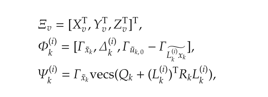
where Xv=vecs(Xm),Yv=vec(Ym),Zv=vecs(Zm),Xm∈ Rn×nand Zm∈ Rm×mare symmetric matrices,Ym∈Rm×n,k∈[k0,N).

We first prove property 1).Obviously,Φ(i)has full column rank if and only ifhas full column rank for all k∈[k0,N).This is equivalent to show that linear equation

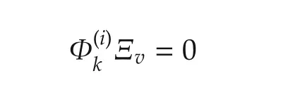
has unique solution Ξv=0.We shall show that it is indeed the case.

According to the definition ofand the equation(24),we have

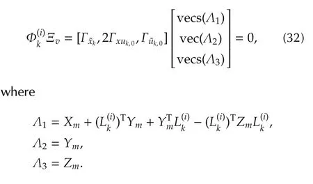
From(31),we know that[Γxk,2Γxuk,0,Γuk,0]has full column rank.This means the only solution to(32)isΛ1=0,Λ2=0,Λ3=0.This is true if and only if Ξv=0.Thusalways has full column rank.Therefore,Φ(i)has full column ranks for all i∈Z+.

Now we prove property 2).By(24),it is easy to check that

Suppose now Ξvand symmetric matrix Wm∈ Rn×nsatisfies

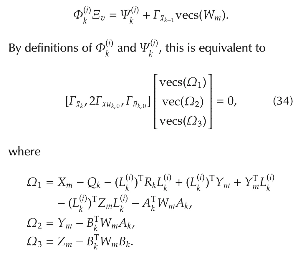
Again,[Γxk,2Γxuk,0,Γuk,0]has full column rank.This means the only solution to(34)is Ω1=0, Ω2=0,Ω3=0.Substituting Ym=BTkWmAk,Zm=into Ω1=0,we obtain

which is exactly the Lyapunov equation(12).SinceF for all i∈Z+,Policy Iteration by(27)and(13)is equivalent to(12)and(13).By Theorem 1,the convergence is proved.

Remark 7 Different from the infinite-horizon PI algorithms[30,31,35,39],where the initial gain matrices must be stabilizing to guarantee the convergence of the algorithm,there is no restriction on the initial gain matrices in finite-horizon PI-based ADP.However,in practice,utilization of stabilizing initial gain matrices(if exist)will prevent the system states from becoming too large.This is beneficial for the sufficient excitation of the systems and numerical stability.

4.2 VI-based off-policy ADP

In this section,we develop a VI-based off-policy ADP scheme using(5).

For k=k0,...,N-1,define

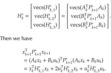
Similar to the last section,suppose l groups of different control(26)are applied to the systems to collect data.Above equation yields

Theorem 4 If there exists an integer l0＞0,such that,for all l＞l0and k∈[k0,N),(31)holds,then Algorithm 2 yields the optimal values

Remark 8 In this paper,two data-driven ADP methods are proposed.Compared with PI,VI is much easier to implement and only requires finite steps to find the optimal solution.However,all the(N-k0)-step iterations must be executed cascaded to find the optimal solution,which is time consuming when N is large.On the contrary,in PI,the full sequencecan be obtained in each learning iteration in parallel.Due to the fast convergence of PI,PI shows a better performance when N is large.

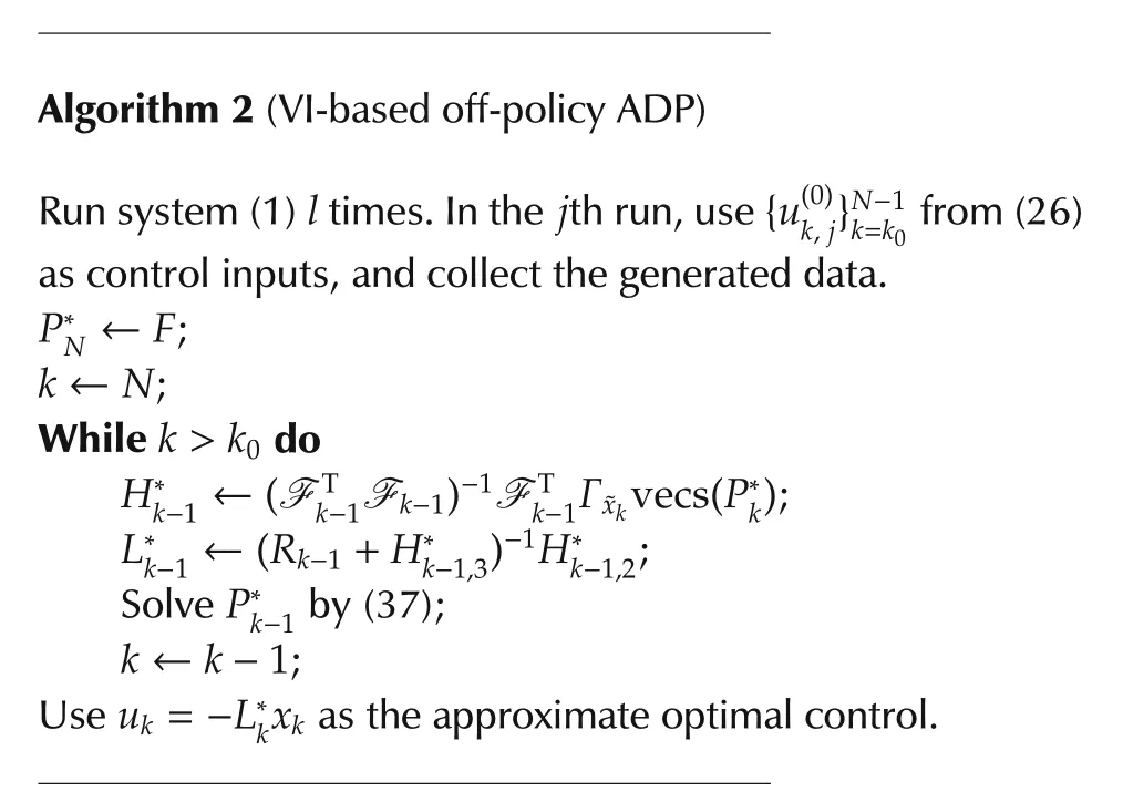
Algorithm 2(VI-based off-policy ADP)Run system(1)l times.In the j th run,use{u(0)k,j}N-1 k=k0 from(26)as control inputs,and collect the generated data.P＊N ←F;k←N;While k＞k0 do H＊k-1←(F T k-1 F k-1)-1 F T k-1Γxk vecs(P＊k);L＊Solve P＊k-1 by(37);k-1←(Rk-1+H＊k-1,3)-1 H＊k-1,2;k←k-1;Use uk=-L＊k xk as the approximate optimal control.

5 Application

In this section,we apply the algorithms presented in previoussectionsto the spacecraftattitude controlproblem.Due to a space structure extended in orbit[40]or on-orbit refueling[41],moment of inertia of the spacecraft will be time-varying.This can be modeled by the following continuous-time linear time varying system[42],

where x=[q,˙q]T,q=[α,β,γ]T,α,β,γ are the row angle,the pitch angle,the yaw angle of spacecrafts respectively,

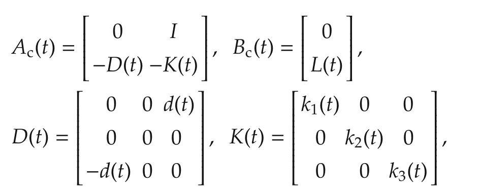
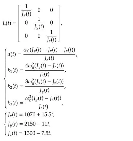
Jx(t),Jy(t),Jz(t)are the components of momentof inertia of spacecrafts with respect to a body coordinate system,and ω0=0.0011 rad/s is the orbital rate.We discretize system(38)by using Forward-Euler method with sampling time h=0.1 s,and obtain the discrete-time linear time varying system,

Let final time N=300,and choose weighting matrices Q=10I6,R=I3.The proposed Algorithms 1 and 2 are applied to system(39).For Algorithm 1,the initial control gains are all zero matrices.To collect data that satisfies conditions(31),in the simulation,the elements of initial angles q0are assumed to be independently and uniformly distributed over[-1,1],while the elements of initial angle velocities˙q0are assumed to be independently and uniformly distributed over[-0.01,0.01].The exploration noises are chosen as

where for r th component of control input,in j th trial,each σs,jis independently drawn from the uniform dis-tribution over[-500,500].

Algorithm 1 stops after 10 iterations on this task.Fig.2 shows the convergence ofin the PI case.One can find that,for fixed time k,converges monotonically to their optimal values,as predicted in Theorem 1.For Algorithm 2,the maximum difference between the LS solutionsgiven by Algorithm 2 and the optimal values P＊k,measured by matrix 2-norm,is 1.6749×10-8.The final approximate optimal control gains and the initial control gains(all zero matrix)are applied to system(39)with initial condition q0=[0.0175,0.0175,0.0175]T,˙q0=[0,0,0]T.The state trajectories under these two control are shown in Figs.3 and 4,respectively.The final control inputs are shown in Fig.5.Therefore,the simulation results demonstrate the effectiveness of the proposed finite-horizon PI and VI algorithms.

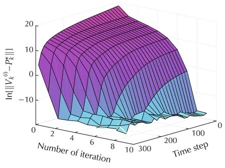
Fig.2 Comparison of with its optimal value.

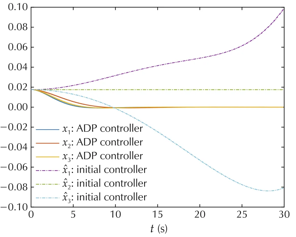
Fig.3 Trajectories of angles of the spacecraft.

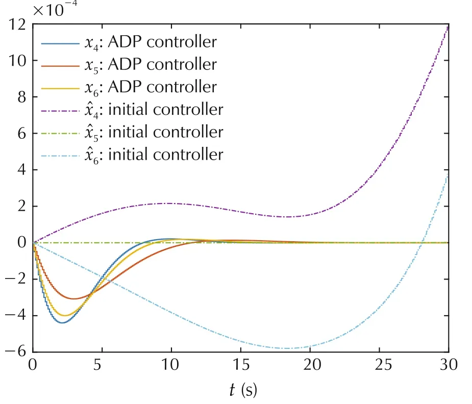
Fig.4 Trajectories of angle velocities of the spacecraft.

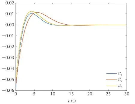
Fig.5 Approximate optimal control inputs.

6 Conclusions

The popular policy iteration(PI)method has been extended for the finite-horizon optimal control problem of linear time-varying discrete-time systems in this paper.In the stationary case,its connections with the existing infinite-horizon PI methods are revealed.In addition,novel data-driven off-policy PI and VI algorithms are derived to find the approximate optimal controllers in the absence of the precise knowledge of system dynamics.It is shown via rigorous convergence proofs that under the proposed data-driven algorithms,the convergence of a sequence of suboptimal controllers to the optimal control is guaranteed under some mild conditions.The obtained results are validated by a case study in spacecraft attitude control.