Distributed adaptive Kalman filter based on variational Bayesian technique
2019-01-24ChenHUXiaomingHUYiguangHONG
Chen HU ,Xiaoming HU ,Yiguang HONG
1.Rocket Force University of Engineering,Xi’an Shannxi 710025,China;
2.Department of Mathematics,Royal Institute of Sweden(KTH),Sweden;
3.Institute of Systems Science and University of Chinese Academy of Sciences,Chinese Academy of Sciences,Beijing 100190,China
Received 31 August 2018;revised 23 October 2018;accepted 23 October 2018
Abstract In this paper,distributed Kalman filter design is studied for linear dynamics with unknown measurement noise variance,which modeled by Wishart distribution.To solve the problem in a multi-agent network,a distributed adaptive Kalman filter is proposed with the help of variational Bayesian,where the posterior distribution of joint state and noise variance is approximated by a free-form distribution.The convergence of the proposed algorithm is proved in two main steps:noise statistics is estimated,where each agent only use its local information in variational Bayesian expectation(VB-E)step,and state is estimated by a consensus algorithm in variational Bayesian maximum(VB-M)step.Finally,a distributed target tracking problem is investigated with simulations for illustration.
Keywords:Distributed Kalman filter,adaptive filter,multi-agent system,variational Bayesian
1 Introduction
In recentyears,distributed estimation design ofmultiagent systems has received more and more attention,because of its broad range of applications in engineering systems such as communication networks,sensor networks,and smart grids.Distributed Kalman filter(DKF)is one of the important distributed estimation methods,which plays a key role due to its power of real-time estimation and non-stationary process tracking[1-7].For example,R.Olfati-Saber[1]constructed DKF by putting the consensus terms in each Kalman filter update step,while S.Stankovi’c et al.[2]considered the problem for missing observations and communication faults.Also,D.Casbeer et al.[3]and[4]applied consensus algorithms to an information filter,where the unbiasedness and convergence were shown,and W.Yang et al.[7]considered the problem of link acti-vation with power constraints.Moreover,G.Battistelli and L.Chisci[5]considered DKF with consensus on the inverse covariance matrix and the information vector,while Z.Zhou etal.[8]studied DKF for switching communication topologies.However,these works are based on a prior knowledge of measurement noise statistics.
For several decades,various centralized designs of adaptive filters have been proposed to solve the problem with unknown noise statistics,mainly based on the maximum likelihood or covariance matching methods[9-11],which are computationally complex or analytically intractable[12,13].On the other hand,variational Bayesian(VB)methods have been proposed for approximating posterior distribution,which have benefits of low computational cost and analytic tractability[14].Therefore,S.Sarkka and A.Nummenmaa[13]used a VB method to approximate the joint posterior distribution of the dynamic state and measurement noise parameters in linear dynamics,where the variational distribution of noise is assumed as the product of the Inverse-Gamma distributions.Moreover,H.Zhu etal.[15]employed VB to estimate the joint distribution of state and non-Gaussian noises statistical,where the non-Gaussian noise was modeled by Gaussian mixture models.Additionally,P.Dong et al.[16]considered an adaptive VB filter based on the Wishart distribution,to estimate the full noise variance matrix with a fusion center.However,none of these algorithms is applicable to distributed design of multi-agent networks.To the best of our knowledge,the distributed adaptive VB Kalman filters have not yet been adequately investigated,and very few studies on adaptive design for distributed state estimation with unknown measurementnoise variance,though many effective distributed Kalman filters have been developed.
In this paper,we investigate the distributed adaptive VB Kalman filter with unknown noise variance modeled by the Wishart distribution in a multi-agent network.With communication with neighbors,the posterior distribution of joint state and noise variance is approximated by a free-form distribution,where the approximation can be achieved by recursively performing VB-E and VB-Msteps[14].The main contribution ofthe paper can be summarized as follows.A distributed adaptive VB Kalman filter is proposed,which can be viewed as a distributed extension of the centralized one given in the linear case[16].The analysis shows that VB-E step can be achieved only with the local information and the VB-M step can be achieved with a consensus algorithm,where the VB-M structure is consistent with some distributed Kalman filters in[3,4],and then the convergence of the proposed algorithm is proved.
The remainder of the paper is organized as follows.Section 2 presents problem formulation of this paper.Then Section 3 gives the design and analysis of the distributed adaptive VB Kalman filter,and Section 4 shows simulation examples.Finally,Section 5 provides concluding remarks.
Notations N(x;x,P)denotes the Gaussian distribution with meanx and covariance P.diag{·}represent the diagonalizations of block or scalar elements.An undirected graph of N nodes is denoted as G={V,ℰ}with V=1,...,N.The neighbors of node i can be represented by the set{j∈V|(i,j)∈ℰ}≜ Ni,whose size is denoted as|Ni|.
2 Problem formulation
Consider the following stochastic dynamics:

with xk∈Rnas the state observed by a N-agent network G,Ak∈ Rn×nas the system matrix,and wk∈ Rnas the zero-mean Gaussian noise,with E{wkwTk}=Qk.The measurement model is given as

with yi,k∈Rmias the measurement of agent i,Ci,kas the observation matrix of agent i,and vi,k∼N(vi,k;0,Ri,k)as the observation noise.Suppose thatand E{vi,kwTk}=0,∀i∈ V at each k,and all yi,k,∀i∈ V are conditionally independent of given xk.
In the Bayesian filter framework,the dynamics(1)and measurement mapping(2)can be written as state transition probability p(xk+1|xk)and measurement likelihood function p(yi,k|xk),i=1,...,N.Hence,the joint likelihood function is the product of local likelihood functions,

The following assumptions have been widely used in the DKF literature[1,3-6].
Assumption 1 The undirected graph G is connected.
Assumption 2(Collective observability) The pair(Ak,Ck)is observable,where
Since yi,kneeds to be purely nondeterministic and Di,kRi,kDT>0 is a sufficient condition for this,we as
i,ksume Di,k=I,∀i without loss of generality.
Most Kalman filter designs are based on the assumption that Ri,kis known.However,this assumption may not hold in practice,and here we consider the case when Ri,kis unknown.To be strict,we assume that the measurement information matrix Φi,k=follows the Wishart distribution W(Φi,k;νi,k,Vi,k)with parameters νi,kand Vi,k.Note that the Wishart distribution is a conjugate prior for the unknown information matrix of a Gaussian model with a known mean,which is suitable to model the unknown noises[17].
Distributed Kalman filters[1-6]were proposed in(1)and(2)with known Ri,k.However,inaccurate Ri,kmay enlarge the estimation error or even causing divergence.Therefore,we aim at the design of a distributed Kalman filter with unknown measurement noise to estimate the joint posterior distribution p(xk,Φk|Yk)by a network of N agents,where Φk=diag{Φ1,k,...,ΦN,k}.
Remark 1 For comparison,let us define a centralized estimate xckassociated with measurement Yk.Then the centralized estimation consists of the prediction xck=E{xk|Yk-1}and the update xck=E{xk|Yk}.For linear dynamics(1)and measurement equation(2)the well-known Kalman filter gives a recursive solution as follows[18]:
Measurement update:
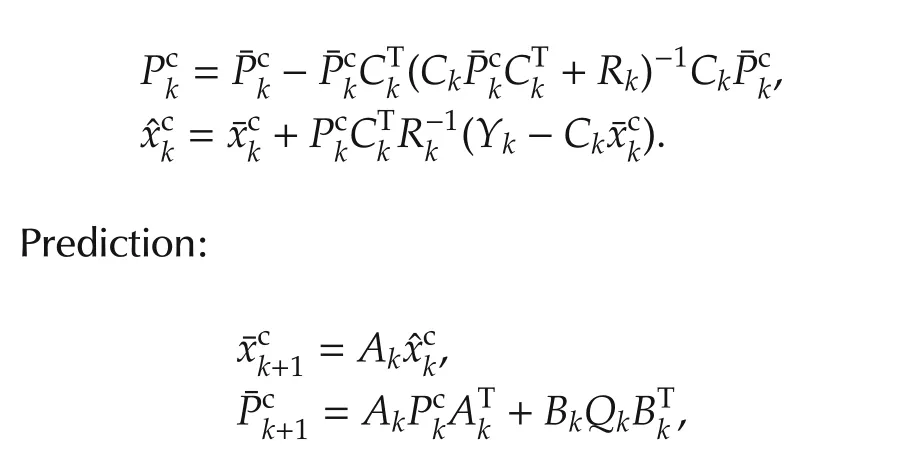
where Rk=diag{R1,k,...,RN,k},and PckandPckare estimate errorcovariance matrices ofxckandxck,respectively.
Suppose that the posterior distribution of xk-1and Φk-1conditional on Yk-1at time k-1 is approximated by

The first equation holds since xk-1and Φk-1are conditionally independent given Yk-1.Note that the form of posterior distribution p(xk,Φk|Yk)remains the same if the predictive distribution p(xk,Φk|Yk-1)is Gaussian-Wishart[19].
The predictive distribution of state xkand Φkare separable and independent,and can be given by the Chapman-Kolmogorov equation,
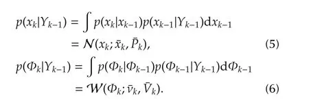
Prediction(5)for(1)results in a Gaussian distribution for predicted xk,with parameters xk=Akxk-1and Pk=AkPk-1ATk+BkQkBTkgiven by the standard Kalman filter prediction equations.
Similar to[13,16],we take the dynamics of Φi,kto ensure that the predictive distribution p(Φk|Yk-1)is Wishart,with ν= μνand V=Clearly,
kk-1kthe value μ=1 indicates a stationary variance,while 0<μ<1 indicates that the variance is time-varying[13].
Because xkand Φkare independent,the prediction for the joint of xkand Φkcan be written as

Based on the standard VB method[14,20,21],the joint posterior distribution p(xk,Φk|Yk)can be approximated by a free-form distribution q(xk,Φk),

where q(xk)and q(Φi,k)are the Gaussian and Wishart distributions,respectively.The VB approximation is achieved by minimizing the Kullback-Leibler(KL)divergence between the posterior distribution p(xk,Φk|Yk)and the variational distribution q(xk,Φk),
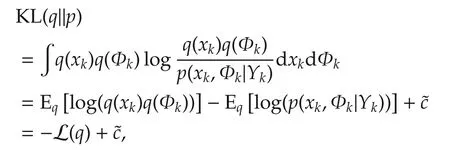
wherec denotes the terms independentofthe variational distribution q(xk,Φk),and

is called the evidence of lower bound(ELBO).
Therefore,our problem becomes

which is equivalent to the minimization of KL(q||p).
The VB approach updates each local variational distribution q(Φi,k)(VB-E step)and the global variational distribution q(xk)(VB-M step)alternatively,with keeping the other distributions fixed:

Note that the estimatexkin(12)can be obtained by each agent if each agent knows the global likelihood function p(yk|xk)[13,15,16].However,in our paper,each agent can only access to its local likelihood function p(yi,k|xk),and thus,we have to propose a distributed adaptive VB Kalman filter to optimize KL(q||p).
3 Distributed adaptive VB Kalman filter
In this section,we discuss the VB approximation of the posterior distribution p(xk,Φk|Yk)in a distributed way,and propose a distributed adaptive VB Kalman filter algorithm(DAVBKF).
Define a set of variables{xi,k,i=1,...,N}for each agent,and let s be the number of VB iterations.Then the approximation distributionsandat the s th step can be given as follows:

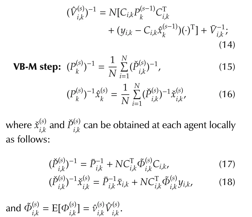
The proposed VB algorithm updates q(Φi,k),∀i∈ V and q(xk)alternatively while keeping the other fixed,to be discussed in Lemmas 1 and 2.
In(13)and(14),each agent only needs the local information in VB-E step.Nevertheless,in VB-M step,a global estimate is achieved by averaging local information of all agents.To computea distributed way,denote

Based on the average consensus algorithm[22],each agent approximatesas follows:
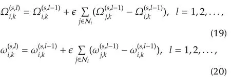
where ϵ is a consensus rate parameter within the range ofwith Δ =max|N|[22].Then we give ouriiDAVBKF in Table 1,with initial conditionand Pi,0=P0.
In the DAKFVB,the initialization of all local estimates is exactly the same mean of the initial state,which is not easy to satisfy in practice.In fact,a practical initialization can be obtained by letting xi,0=0,∀i∈V and Pi,0=0,∀i∈ V,which means that no prior information available.
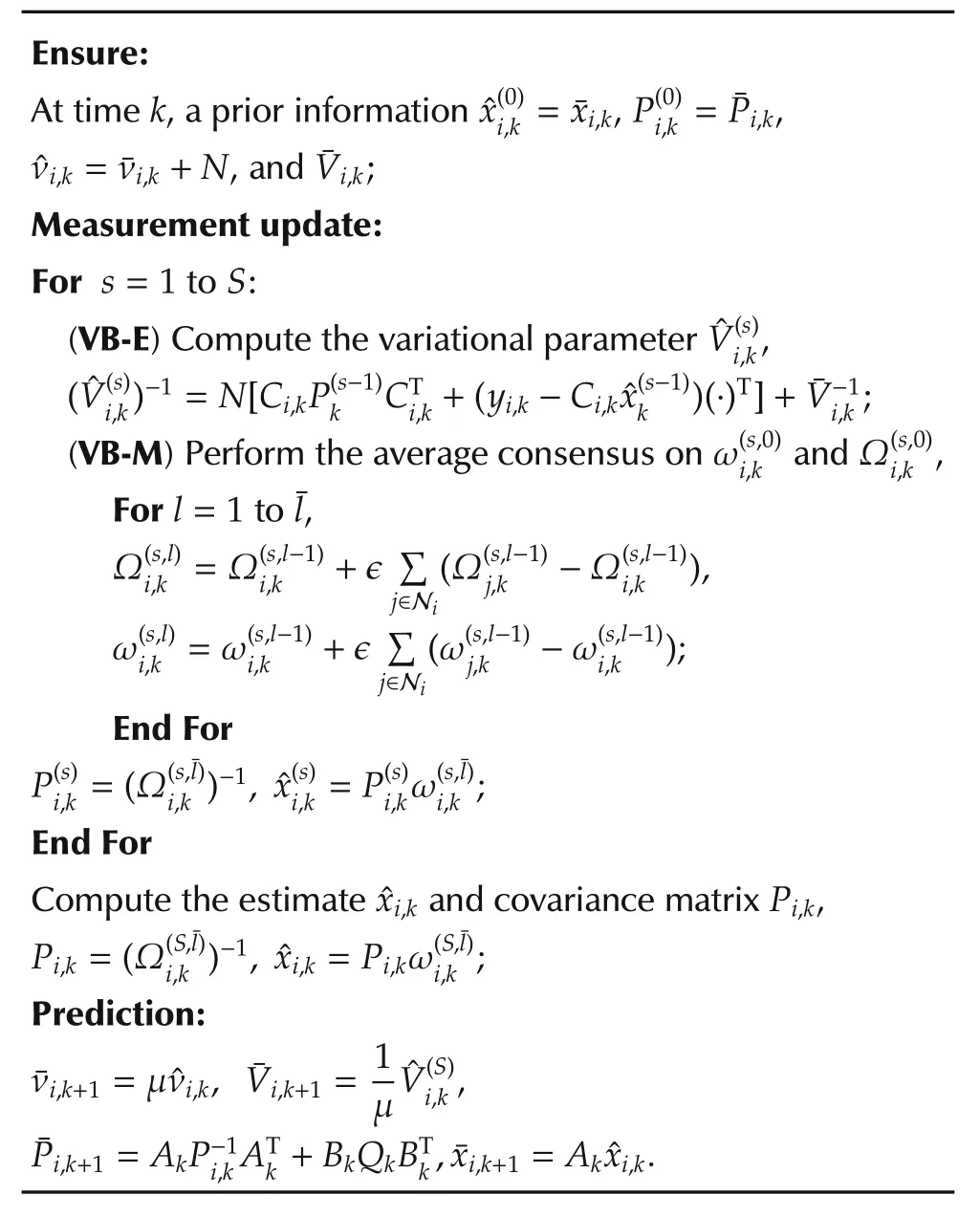
Table 1 DAVBKF at node i at time k.
Remark 2 Note that,in the DAVBKF,the distributed realization of VB approach for q(xi,k)with fixed q(Φi,k)is consistent with distributed Kalman filters in[3,4].Namely,equations(19)and(20)perform measurement updating step of distributed Kalman filters in[3,4]for given noise variance matrices.
Next,we give two lemmas about q(xk)and q(Φi,k),i=1,...,N.The first lemma is for the solution of the variational distribution q(Φi,k).
Lemma 1(VB-E) Given the global variational distribution q(xk;xk,Pk),q(Φi,k;νi,k,Vi,k)of each agent is obtained as follows:
Its proof is in the appendix.
Remark 3 S.Sarkka et al.[13,16]presented adaptive VB Kalman filters.Note that[13]assumed that the measurement noise variance Rkwas a diagonal matrix with a priori distribution of noise modeled as a product of Inverse-Gamma distribution,i.e.,Rk=diag{σk,1,...,σk,m}andwhere IG(σ;α,β)stands for the Inverse-Gamma distribution covered by the parameters α and β.P.Dong etal.[16]presented an adaptive VB Kalman filter for nonlineardynamics,with the noise variance matrix modeled as a Wishart distribution,which resulted in full noise variance matrix estimation.Clearly,VB-E step in Lemma 1 is different from the centralized one in[16],even though(21)and(22)can be obtained by each agent individually.With N=1 in Lemma 1,(21)and(22)will reduce to the VB-E step in[16].
According to the VB approach,an optimal solution of q(xk;xk,Pk)can be achieved by giving q(Φi,k;νi,k,Vi,k),i=1,...,N.However,in a distributed structure,it cannot be solved straightforwardly because each agent cannot access the joint likelihood function p(yk|xk)=of non-neighboring agent.
Since the agents are independent,the posterior can be written asDecomposition of L(q)can be obtained by substituting p(xk,Φk|Yk)into(9).Namely,
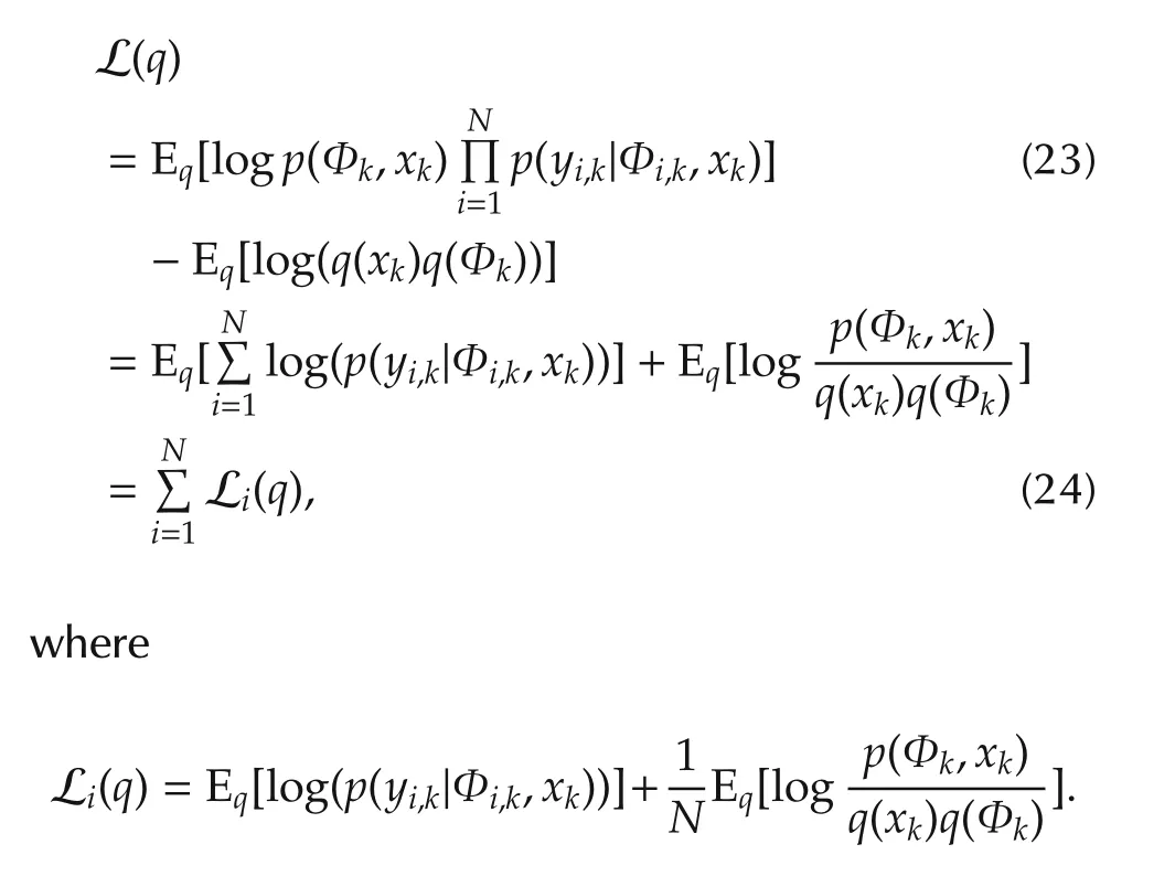
Denote q*(xk;xk,Pk)as an optimal variational distribution for L(q),and,xˇi,k,Pˇi,k)as an optimal variational distribution for Li(q).The next lemma gives the solution for global variational distribution q*(xk),and the relationship with
Lemma 2(VB-M)Suppose that each agent gets the global optimal solution q(xk-1;xk-1,Pk-1)at time k-1.Given q(Φi,k;νi,k,Vi,k),i=1,...,N,q(xk;xk,Pk)can be achieved as follows:


whereˇxi,kandˇPi,kcan be obtained locally as follows:

Its proof is in the appendix.
Then it is time to give our result for the proposed algorithm for an N-agent network.
Theorem 1 Under Assumptions 1 and 2 for the proposed DAVBKF,if each agent is initialized by letting=E{x0}and Pi,0=P0,∀i∈V,then the estimatesconverge to an estimate of centralized solu-tion of(9)as l→∞for all k.
Proof Suppose that,at time k-1,the estimates q(xi,k-1),∀i∈ V of each agent achieve consensus,i.e.,and Pi,k-1=Pj,k-1=Pk-1,∀i,j∈V.In the prediction of the proposed algorithm,we haveand.Therefore,and
The VB approach for measurement update can be achieved by iteratively updating the VB-E and the VB-M steps in DAVBKF.Next,we show the optimality and stability of VB-M step in DAVBKF.At the s th iteration of VB,under Assumption 1,the consensus iterations(19)and(20)converge to the average of(Pˇi,k)-1and(Pˇi,k)-1xˇi,kas l→ ∞[22],respectively.Therefore,
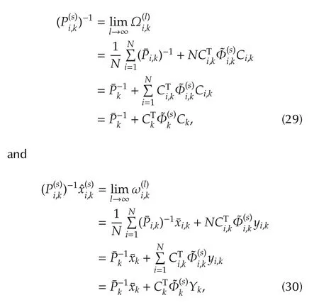
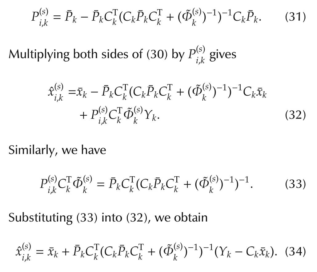
Note that(31)and(34)exactly are the measurement update equations of the standard Kalman filter with measurement noise variance.By Assumption 2,the optimality and stability ofw ith givenare guaranteed.Clearly,as l→ ∞after the VB procedure,which satisfies the conditions of Lemma 2.
According to Theorem 2.1[14],Lemma 1 and Lemma 2,proposed DAVBKF converges to a local maximum of L(q)at time k.This convergence further guarantees that the local optimal centralized estimate will be reached at next step.Thus,DAVBKF withl→∞at each time step can converge to an estimate of centralized solution with initial conditions.
Theorem 1 shows that the global variational distribution q(xk)can be achieved by averaging of a local optimal solution,and the updating of variational distributions q(Φi,k)only need local information of agent i.However,it is not easy to obtain the bound of estimate error,since the VB iteration can only converge to a local optimal solution,and it depend on the estimation at each instant.
Remark 4 The VB approach guarantees the local convergence by iterations of the VB-E and VB-M steps[14].The measurement update in DAVBKF consists of VB-E and VB-M steps,which leads to a fixed point iteration[23],while the prediction in DAVBKF is the same as the prediction step of standard Kalman filter.Moreover,with the collective observability assumption,the dynamics(1)need not be observable by each agent in our analysis.
Remark 5 In Theorem 1,for every k,q(xi,k)of each agent should reach a consensus,asl→∞.In practice,when 0<l<∞,it has been shown that Pi,k,∀i∈ V,k=1,2,...is upper bounded by a positive definite matrixPi,kfor given noise statistics in[3].Recall Theorem 2.1 in[14],the iterations of VB-E(Lemma 1)and VB-M(Lemma 2)steps converge to a local maximum of L(q),which implies that both of Pi,kandΦi,kare bounded.However,in this case,Pi,kwill not represent the error covariance matrices.The simulation part illustrates that DAVBKF can converge fast even ifl=1.
The centralized solution of VB procedure for measurement updating step can be easily obtained by letting N=1 in Theorem 1,which is mentioned in the following result.
Corollary 1 Let s be the iterative number of VB.Assume there exists a center who can access Ckand yk,then VB procedure for optimizing L(q)in(9)can be achieved by the following updates:
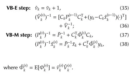
Remark 6 Corollary 1 is consistent with the result in[16].Also,the VB-M step in Corollary 1 is exactly the measurement updating step of the information form of the Kalman filter[18]with a given measurement noise variance.
4 Simulation
Theorem 1 considered the DAVBKF,withxi,0=E[x0],∀i∈V andPi,0=P0,∀i∈V.The VB algorithm alternatively updates each local variational distribution q(Φi,k)and the global variational distribution q(xk).In many simulation examples,the algorithm converges very fast,and only 2 or 3 iterations are good enough in practice.
Consider a target tracking problem,where the target moves with a constant velocity,whose dynamics[24]is
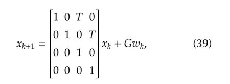
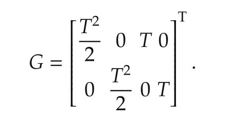
where xk=[dx,dy,˙dx,˙dy],dxand dydescribe the target position,and˙dxand˙dydescribe the target velocity.wk∼N(0,Qk),Qk=diag{[w21w22]}with w21=w22=0.1.T=1s is the sampling period,and
Suppose that the target position can be measured by a network of sensors,whose measurement equations are

The measurement matrices Ci,i=1,...,N satisfy Assumption 2,of the following form

The topology of communication network is shown in Fig.1.
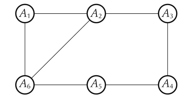
Fig.1 Topology of the network.
The target trajectory is generated by(39)with the initial state x0= [0 0 2 2]T.The initial state of each agent isxi,0=x0+[10 10 5 5]T,∀i∈V andPi,0=diag{[1021025252]},∀i∈V.The true measurement noise variance generated by Ri,k=0.2+0.4(1+tanh(0.1T(k-Tf/4))),k=1,2,...,where Tf=500 is total simulation time.The fading parameter is μ=0.9 for all agents.The initial parameters for q(Φi,0)are νi,0=1 and Vi,0=7.5,i∈V.The number of recursive VB steps is S=3.
Compare the performance of the DAVBKF with a centralized adaptive VBKalman filter(CAVBKF),which isthe linearcounterpartthe one given in[16](see Corollary 1),by conducting numerical simulations,where 200 Monte Carlo trials for the CAVBKF and the DAVBKF are performed,respectively.In the CAVBKF,the measurement matrix is C=Tand Rk=diag{R1,k,...,R6,k}.
Consider the mean square estimation errors(MSE),which has been widely used for the estimator performance,

In order to compare the estimation errors of the noise variances,we define the total estimate errors of noise variance as

Figs.2 and 3 show the MSEs of position and velocity,respectively.DAVBKF-1 and DAVBKF-100 represent the numbers about consensus arel=1 andl=100 for the DAVBKF,respectively.It can be seen that the MSE of DAVBKF-1 is little larger than that of the MSE of DAVBKF-100.However,the DAVBKF performs better than the CAVBKF even whenl=1.Fig.4 shows the estimates ofnoise variance fordifferentagent,and Fig.5 shows the estimation errors of measurement noise variance between DAVBKF-100 and the CAVBKF,which demonstrates that the DAVBKF can outperform the CAVBKF.
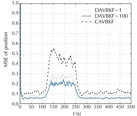
Fig.2 MSE of position.
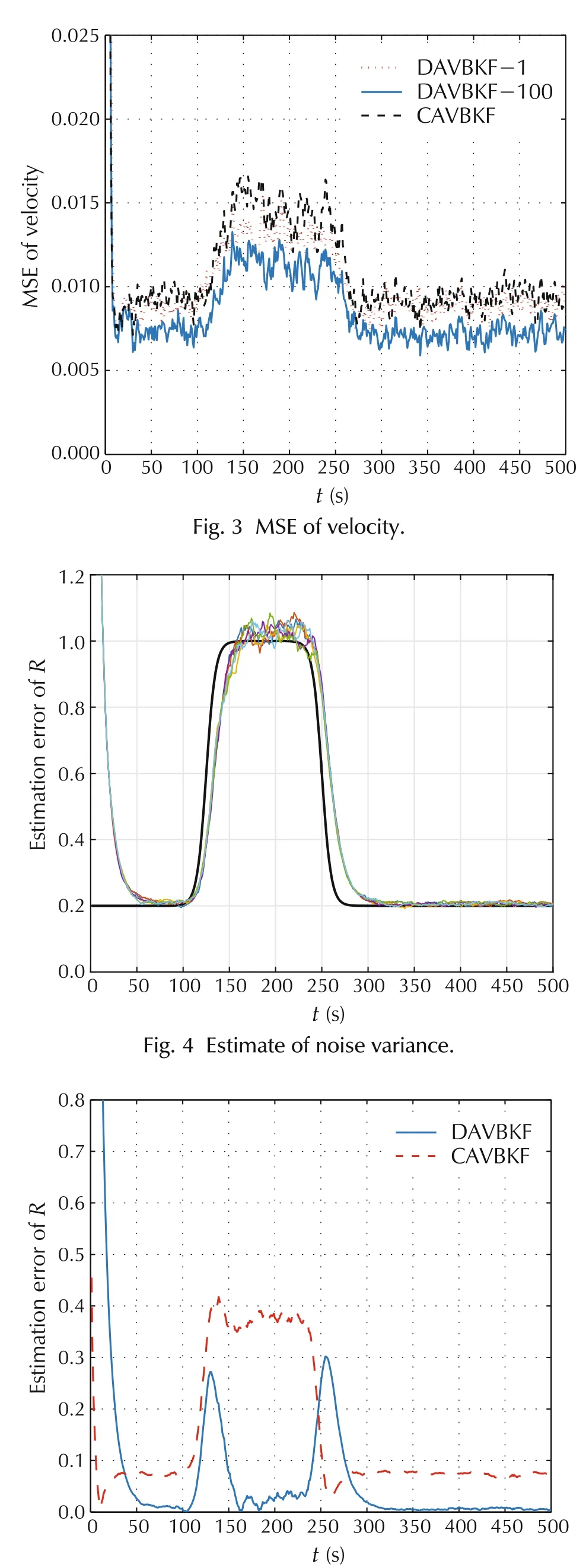
Fig.5 Estimate errors of noise variance.
A reason why the DAVBKF performs better than the CAVBKF is that the global ELBO L(q)over the whole network may less than the summation of the local ELBO Li(q)over each agent[25],i.e.,,which shows that the DAVBKF may perform better than the CAVBKF.
5 Conclusions
In this paper,a distributed adaptive VB Kalman filter was investigated with unknown measurement noise variance modeled by the Wishart distribution.The posterior distribution of the joint state and noise variance were approximated by a free-form variational distribution.Itwasshown thatthe estimate ofthe noise variance only depended on the localinformation and the estimate could be achieved by a consensus algorithm based on VB.In the numerical simulations,the distributed tracking problem was studied,which verified and showed the effectiveness of the proposed algorithm.
Appendix
Proof of Lemma 1 Clearly,with qi≜ q(xk)q(Φi),
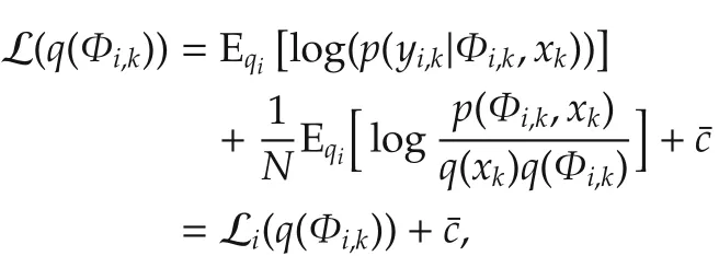
wherec denotes a constant independent of Φi,k,and Li(q)is defined in(24).For fixed q(xk),the variational distribution q(Φi,k)only related to the local measurement yi,k,and thus,it can be solved individually by each agent.
Then the conditional distribution p(yi,k|Φi,k,xk)is
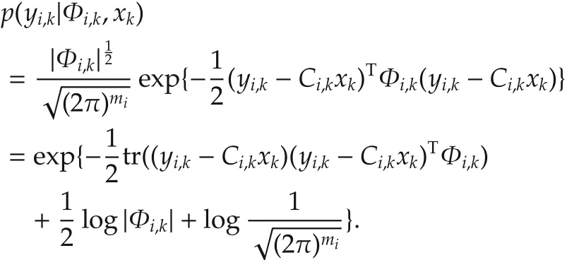
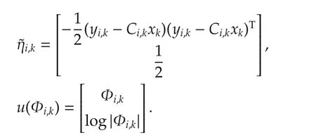
Rewrite the following probability densities in the exponential family form[26].Denote the natural parameter of q(Φi,k)is ηi,k,and corresponding sufficient statistical and log-normalizer are u(Φi,k)and Al(η),respectively.Rewrite Li(q(Φi,k))in the exponential family distribution form:

wherec1is a constant independent of Φi,k,andηi,kand Al(ηi,k)are natural parameter and log-normalizer of W(Φi|νi,k,Vi,k),respectively.and u(Φi,k)are given by1Notice that we use tr(MN)=vec(M)·vec(N),and then vectorizing the matrix parameter when inserted into the exponential family form.
By taking the derivative of Li(q(Φi,k))with respect toηi,k,we have

due towe have the solution of natural parameters of q(Φi,k),

Note that
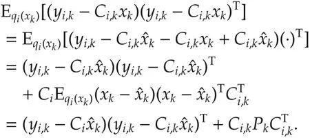
Thenare given by

Proof of Lemma 2 Clearly,

and then

wherec0denotes the terms independent of xk.
Rewrite

where the natural parameter of a Gaussian distribution
Substitute equations(a3),(a4)and(a5)into Li(q),
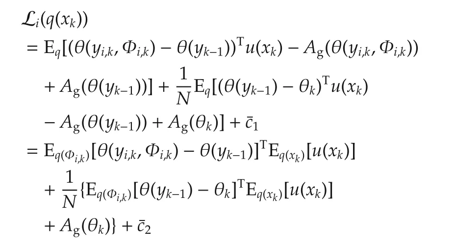
due to the exponential family propertyAg(θk),wherec1andc2are the terms independent of xk.
Taking the derivative of Li(q(xk))with respect to θkgives

Then the global optimal solution can be found by lettingwhich yields

With a similar procedure,the local optimal solution can be given as

Combining(a6)and(a7)yields

Since p(xi,k|yi,k,Φi,k)and p(xi,k|yi,k-1)are Gaussian distributions,be given as

whereΦi,k=Eq(Φi,k)[Φi,k]=νi,kVi,k.With(a8),(a9),and(a10),the conclusions follow.
杂志排行
Control Theory and Technology的其它文章
- A new semi-tensor product of matrices
- Precedence-constrained path planning of messenger UAV for air-ground coordination
- Prediction method for energy consumption per ton of fused magnesium furnaces using data driven and mechanism model
- Axis-coupled trajectory generation for chains of integrators through smoothing splines
- An output-based distributed observer and its application to the cooperative linear output regulation problem
- Adaptive dynamic programming for finite-horizon optimal control of linear time-varying discrete-time systems
