Axis-coupled trajectory generation for chains of integrators through smoothing splines

Shupeng LAI,Menglu LAN ,Kehong GONG ,Ben M.CHEN 3,

1.Department of Electrical and Computer Engineering,National University of Singapore,Singapore 117583;

2.Graduate School for Integrative Science&Engineering,National University of Singapore,Singapore 119077;

3.Department of Mechanical and Automation Engineering,The Chinese University of Hong Kong,Shatin,N.T.,Hong Kong,China

Received 18 September 2018;revised 26 October 2018;accepted 29 October 2018

Abstract Integrator based model is used to describe a wide range of systems in robotics.In this paper,we present an axis-coupled trajectory generation algorithm for chains of integrators with an arbitrary order.Special notice has been given to problems with pre-existing nominal plans,which are common in robotic applications.It also handles various type of constraints that can be satisfied on an entire time interval,including non-convex ones which can be transformed into a series of convex constraints through time segmentation.The proposed approach results in a linearly constrained quadratic programming problem,which can be solved effectively with off-the-shelfsolvers.A closed-form solution is achievable with only the boundary constraints considered.Finally,the proposed method is tested in real experiments using quadrotors which represent high-order integrator systems.

Keywords:B-spline,trajectory generation,chains of integrators

1 Introduction

Chains of integrators are used in approaching and analyzing the dynamics of many systems in robotic applications,such as the electrical motor,robotic arms,and computer numerical control(CNC)machines.Especially,many of the holonomic vehicles,including the recently popularmulti-copters,can be effectively simplified into chains of integrator because of their differential flat properties[1].In many of these applications,it is desirable to generate a trajectory that satisfies certain constraints while minimizing the deviation from a preexisting nominal plan[22].

.Boundary conditions:The trajectory is required to start and end in a specific state.For example,many methods rely on trajectory re-planning to handle the system and environment uncertainties,the initial state in such a problem is usually the current or near future state of the system.

.Input constraints:Most robotic system has limited input,such as limited torque,current,etc.If a trajectory is to be tracked precisely and safely,the limits on inputs need to be satisfied.

.Safety constraints:The trajectory has to stay in certain safe regions.Moreover,in many cases,this leads to non-convex constraints due to the nature of the system or the environment.

.Derivative constraints:Many systems come with state limits that can be expressed as the derivative of the trajectory,such as the maximum angular speed of a motor,the limited acceleration of a multicopter,or the jerk constraint in a CNC machine.

Generally,the last two constraints can also be summarized as the state constraints.In robotic applications,due to the limited computational power and the requirement of real-time capability,they are usually dealt with vastly different methods.

Many systems adopt a multi-layer approach in motion planning to reduce the volume of the search space.Global planning is usually conducted with a vehicle model with highly reduced dynamics,and results in a nominal plan consisting of simple geometric primitives such as points and lines.A trajectory generation algorithm shall be able to minimize the derivative to the nominal plans while satisfying all the above mentioned constraints.Finally,a smooth reference trajectory is usually desirable.It implies a minimized energy consumption and lesser wear and tear,which are beneficial in general.

There is a rich literature on trajectory generation.A common approach is first to generate multiple keyframes which are then interpolated through polynomials.A recent example can be seen in[1],where the authors formulate a(QP)problem to interpolate a series of waypoints using polynomial splines.It can be considered as a multiple shooting method due to the usage of equality constraints to connect different polynomial segments.For chains of integrators,the underlying ordinary differential equations(ODEs)in a shooting method can be solved analytically.Therefore,it is possible to reformulate the problem with different variables and eliminate the unnecessary equality constraints[2].However,due to the base functions used in[1]and[2],they only support point-wise constraints.One needs to enforce the constraints at multiple discrete samples[3]or solve the problems various times[4]to ensure the constraints are well satisfied on the entire trajectory.To address the issue,B’ezier curve is adopted in[5]and[6]to enforce the constraints in a continuous time interval.However,it is not applied to the trajectory’s derivatives,and the equality constraints for segment connection cannot be omitted.

On the other hand,the authors of[10]presents a method based on the pontryagin’s maximum principle to generate a jerk limited and time-optimal trajectory in the form of cubic splines.The method utilizes a decision tree to differentiate between multiple shapes of acceleration profiles where each of them has an analytic solution.Therefore,it is highly efficient,and a trajectory could be generated in micro-seconds level.The author of[7]laterextended itformulti-axis synchronization and applied to robotic arms[8].In[9],the authors adopt a binary searching based approach to simplify the solution of the original problem and extend it to support higher order systems.But the time consumption grows exponentially with the system order and the time optimally is lost.The input reference generated by the methods mentioned above[7,10]always switches between its maximum magnitude and zero.While it is less obvious for electric motors,it could trigger unnecessary aggressive maneuvers for other systems such as the multicopters.Moreover,these methods can only be used to solve two-point boundary value problems instead of a general interpolation.In[21],this method has been successfully implemented on a vertical-take-off-and-landing vehicle.

Furthermore,B-splines have also been used for generating trajectories for chains of integrators.By using the control points as variables,it guarantees the continuity of the trajectory implicitly,and the equality constraints for segment connection can be safely ignored.The formulation presented in[11]and[12]explores the nonnegativity and partition-of-unity properties of the base function to satisfy linear boundaries over a time interval.However,the proposed piece-wise linear boundaries decomposition is only applied to 2-dimensional cases,and it is not sufficient to constrain the trajectory inside arbitrary non-convex regions.Moreover,it fits only point-wise or time-dependent nominal plans but not other geometric primitives.

In this paper,we propose a method based on the B-spline to solve the problems mentioned above with efficient QP formulation.Its major advantages include:

.Addressing the issues of axis-coupling and intervalwise effectiveness through the convex hull property of the B-spline.

.Converting non-convex constraints into convex ones through segmentation.

.Resulting in a QP with adjustable problem size,which offers a trade-off between solution quality and computing time.

Throughoutthe paper,X ∈ Rd×1denotes the d dimensional workspace,where d∈N.For vectors or matrixes,the bracketed subscript denotes specific elements.For a vector a ∈ Rm×1,then a(i)represents its i th element.Similarly,for a matrix A ∈ Rm×n,A(i,j)denotes its element in row i and column j,and A(i,＊)represents the entire i th row,and A(＊,j)represents the entire j th column.For the axis-coupled formulation,the Kronecker product is marked by the⊗operator,and Iddenotes the identity matrix Rd×d.Finally,for a matrix A,its vectorizationA is defined asA=[A(1,＊),A(2,＊),...,A(m,＊)]Twhere T denotes the transpose.

The rest of the paper is organized as follows.The introduction to the B-spline formulation is covered in Section 2;whereas,in Section 3,we show how to formulate the desired problems with quadratic cost functions and linear constraints.In Section 4,the resulting QP is presented,and its solution is discussed,including a closed-form solution.To demonstrate the proposed method,real-experiments are performed using quadrotors,the results and analysis are provided in Section 5.Finally,a conclusion is drawn in Section 6.

2 Background materialon B-spline approximation

B-spline,or the basis spline is widely used in statistics for curve fitting and data differentiation.A k th order B-spline Skcan be expressed as

where Nkiis the basis function and ci∈ Rd×1is called the controlpoint.The basis functionsare defined overan knot vector K=[s0,s1,...,sM+k]and a path parameter s:

where

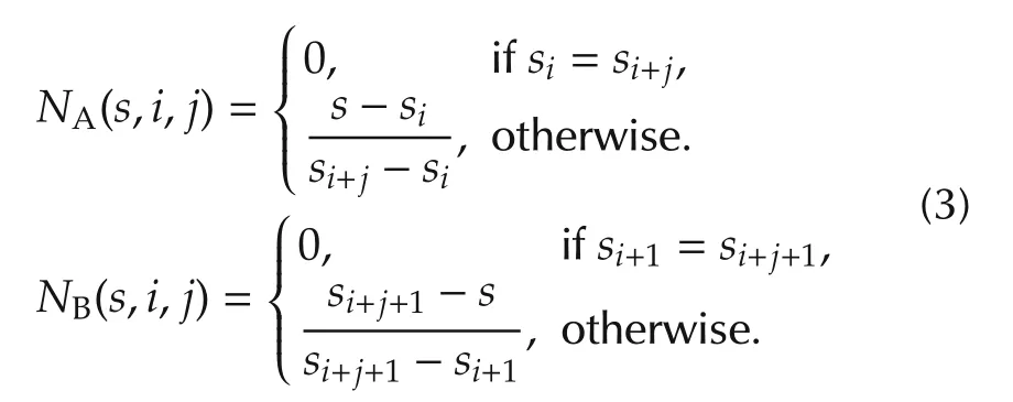
In order to achieve an efficient QP problem,the cardinal B-spline is chosen where the knots have equal distances in between[13].Since most robotic application have boundary conditions to be satisfied,the first and last knots are repeated k times,thus an closed-form solution for boundary value problems can be achieved.Therefore,the knots can be written as

A linear mapping from path parameter s to time t is introduced:

It gives Sk(s)=Sk(αt)where t ∈ [0,Tend]and Tend=The basis of a 4th order cardinal B-spline can be seen in Fig.1.

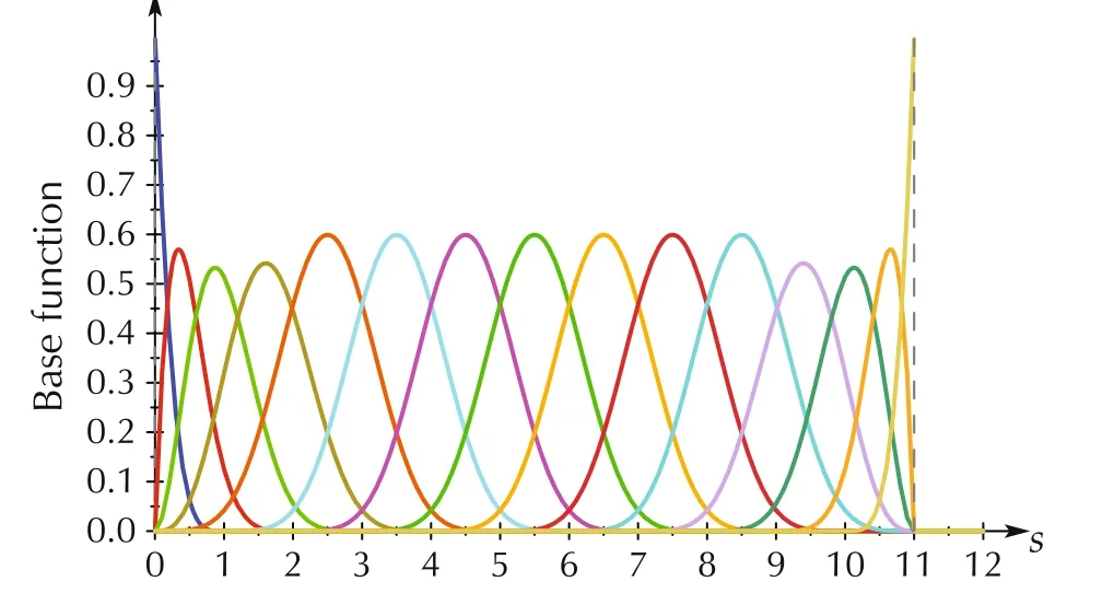
Fig.1 Base function of a cardinal B-spline.

For the ease of analysis,we also define

as the control point matrix.

Due to the selected basis function,the B-spline has the following two important properties:

.Non-negativity:Nki(s)?0 for all i∈{0,1,...,M-1}and s∈[s0,sM+k].The two property together define the convex-hull property and will be used through out the paper.

.Partition-of-unity:

3 Axis-coupled smooth trajectory

In this section,we formulate trajectory generation as an optimization problem.The focusison achieving an efficient QP to fit various geometric primitives,and transforming non-convex constraints into convex ones.With such a simplification,the proposed formulation can be solved with off-the-shelf QP solvers and satisfy the realtime requirement in robotic applications.

3.1 Method overview

The trajectory generation problem can be briefly considered as

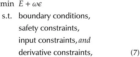
where E stands for the integration of the square of the trajectory’s derivatives;and by minimizing E the trajectory becomes more smooth.The term ϵ represents the deviation from the desired nominal plan.Previously,the description of nominal plan in such a fitting problem is limited to points or keyframes.In this paper,it is extended to cover general geometrical flats in the high-dimensional space.Both E and ϵ can be expressed as quadratic terms related to the control points.Moreover,ω is a weighting factor and all constraints are linear.Among them,the boundary conditions are a set of equality constraints,and the others are sets of inequality constraints.The rest of this section shows how the cost function and the constraints are constructed.

3.2 Smoothness cost

By minimizing the integration of the square of the trajectory’s derivatives,abrupt changes on the trajectory is penalized,and a smoother trajectory is expected.Here the cost function E can be expressed as

where σ(n)?0,∀n ∈ {1,...,k}are the weighting factors.By introducingC,which is the vecorization of the control point matrix C,it can be expressed in quadratic form[11]as

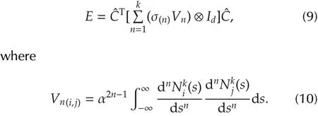
From equation(8),it is guaranteed E?0,therefore σ(n)Vn⊗Idis positive semi-definite.

3.3 Deviation cost

We show how to formulate quadratic cost functions to penalize the deviation from a given nominal plan which includes points,lines,and planes.The presented method can be applied to arbitrary geometric flats in high dimension.

3.3.1 Points

Point and keyframe based nominal plane are widely used in robotics.For a problem in a d dimensional space,a higher level planner would generate a list of NWdesired position-points,each of which is in Rdand to be reached at a specific time-point.Let the i th position-point and time-point be denoted by pi∈Rdand ti∈R with i∈{0,1,...,NW-1}.The cost function shall penalize the distance from the trajectory to the position-points atthe corresponding time-points.Let D=[p0,p1,...,pNW-1]Tand T=[t0,t1,...,tNW-1]T,ti∈R,the cost function can be written as

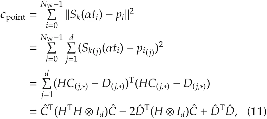
where H ∈ RN×Mis constructed as Here HTH⊗Idis also positive-semidefinite.On the other hand,if the position-points need to be reached exactly,the following equality constraints shall be introduced:

3.3.2 Lines

For holonomic vehicles,the high-level planning algorithm usually produces nominal plans consist of straight lines,which is then sampled into multiple positionpoints in a trajectory generation problem.Here,we present a method to penalize the trajectory’s deviation to straight lines without drawing position-point samples.Assume the high levelplannerproduces NLstraight lines.Whereas the j th straight line passes through the position-points vj,wj∈ Rd,where j∈ {0,1,...,NL-1}.

For a point p∈Rd,the square of its distance to the j th straight line can be written as

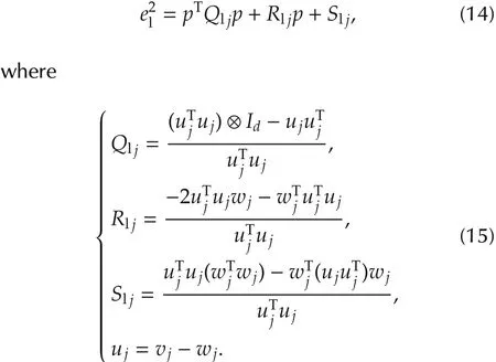
Assume cdis the furthest control point to the straight line,the following shows that the deviation from the trajectory to the straight line will be no further than cd.

Proof Combining equations(1)and(5),a point p on the B-spline at time tsis

For simplicity,we denote Nki(αts)as Niand drop the subscripts for Qlj,Rljand Slj.Then,there is

where Q is positive-semi definite(equation(15)),and there is

Through the non-negativity and partition-of-unity property of the B-spline,there are

Since cdis assumed to be the furthest control point from the straight line,there is

Substitute equations(18)-(21)into(17)produces

Itis then possible to penalize the trajectory’s deviation by minimizing the distance between the control points and the straight line.

3.3.3 Planes

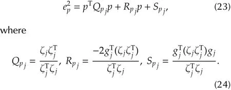
As an example to extend to other higher dimensional flats,we show how to minimize the distance between the trajectory and desired planes.Let the j th plane be defined by a normal vector ζj,an anchor point gj∈ Rd,

where j∈{0,1,...,NP-1}.It indicates a plane contains gjand perpendicular to ζj.Similar to the previous case,it is assumed that the j th plane shall be approached on time-interval[τj,ρj).Then,the square of the distance from a point p to a plane can be written as We could then formulate the cost function to penalize the deviation by minimizing the control points’distance to the plane.

3.4 Time segmentation

Itisusually less meaningfulto approach allthe straight lines or planes simultaneously.Here,we separate them in time by penalizing the deviation to the j th straight line or plane only within a time interval[τj,ρj),where j∈{0,1,...,NL-1}.

From equation(5),the corresponding path variable of a time point τjis ατj,which falls between the knot vector[sη(τj),sη(τj)+1)with η(τj)= ⎿ατj」+k.From equation(3),there are at most k+1 non-zero basis functions on the knot span[ui,ui+1),specifically:Correspondingly,given the time interval[τj,ρj),only the basis functions Nik(s),i∈ {η(τj)-k,...,η(ρj)}can be non-zero.Therefore,we can ignore the control points paired with zero basis functions.

For the NLstraight lines,the cost function to penalize the deviation on their individual time interval can be written as

where λτj= η(τj)-k,λρj= η(ρj),and Λiis a mapping matrix between the vectorization of the control point matrix and the i th control point:

In Section 3.3.2,it shows Qljis positive-semi definite,so does thein equation(25).

Similarly,for the NPplanes,the cost function in equation(23)can be written as

which is also quadratic and convex.

3.5 Deviation from line segments

By combining the time segmentation method with the cost function for the basic geometric flats,it is possible to write quadratic cost to penalize the deviation to more complex geometric primitives.Here,we consider penalizing the deviation to a series of interconnected line segments.Many sampling-based planners would produce such a line-segment based nominal plan.Assume the i th line-segment is defined by two waypoints Wpiand Wpi+1,an example then can be illustrated as in Fig.2.

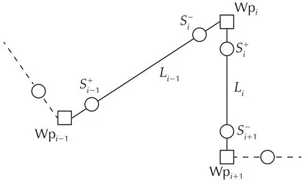
Fig.2 Problem construction of the proposed method.

Due to the reduced system dynamics during higherlevel planning,the waypoints usually are not associated with a time-point.Therefore,we first estimate these time-points using a single or double integrator model,where closed-form solution exists.Assume the time point for the i th waypoint Wpiis tiwhere i∈{0,1,...,NW-1}.Here we adopt the double integrator estimation model,then Δti=ti+1-tiis calculated as the minimum time to move from Wpito Wpi+1along the line Li,with zero boundary velocities,while satisfying the maximum speed vmaxiand the maximum acceleration amaxi.The time optimal trajectory and Δtican be calculated efficiently using the algorithm in[14].Additionally,two intermediate waypointsare selected from the time optimal trajectory at moments ti+κΔtiand ti+(1-κ)Δtiwhere κ is a design variable.These moments also serve as the time-points for S+iandSince the time optimal trajectory always stays onstraight line,so doesThen,to penalize the deviation from the line segments,we minimize:

.The distance to points Wpitheir corresponding time-points.

.The deviation from the underlying straight line Liover[ti+κΔti,ti+(1-κ)Δti)for i∈ {0,1,...,NW-2}.

3.6 Safety constraints

Many robotic applications require the trajectory to stay in certain safe regions which are usually non-convex such asin the case ofobstacle avoidance.However,non-convex optimization is generally difficult to solve,which is against requirements of reliability and efficiency in robotic trajectory generation problem.To address this issue,the non-convex safe region is decomposed into multiple interconnected convex regions through time segmentation.It can be illustrated using the following example.

In Fig.3,the safe region S is originally non-convex.However,itcan be decomposed into multiple convex regions C=[C0,C1,C2].Assume the trajectory is to stay inside S on the timer interval[τ0,τf),we can construct the following sufficient and convex conditions:

which guarantees the trajectory to stay inside S.The example can be extended into higher dimensions with an arbitrary number of decomposed convex regions.Assume the convex regions are all polytopes,where the interior of each can be represented by{p∈Rd|Ajp?bj}with j∈{0,1,...,NC-1}.For the completeness of the paper,we now show that if all control points for a B-spline satisfy

so does the entire trajectory which is commonly called the convex hull property of the B-spline.

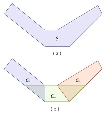
Fig.3 Dcomposing of the non-convex region.(a)Non-convex region.(b)Convex subregions.

Proof Assume that a point p is select from the trajectory at time ts.For simplicity,we use Nito denotethen there is

By the non-negativity and partition-of-unity of the basis functions,and equation(29),

Through the time segmentation,we can assume the trajectory satisfies the j th convex region constraint on the time interval[τj,τj+1).Following the analysis in Section 3.4,it affects a finite subset of the control points,which can be written as Ajci?bj,∀i∈{η(τj)-k,...,η(ρj)}.Combining equation(26),we have the following linear inequality constraints for the safe regions:

3.7 Derivative constraints

In many cases,it is also desirable to constrain the trajectory’s derivatives.Several previous methods[10,15,16]propose to enforce the constraints along each axis,which spans an axis-aligned cuboid.By using the proposed method,it is possible to construct axis-coupled constraints that come with larger interior volume,with which the trajectory could achieve a lower cost.In Fig.4,the desired acceleration constraint spans a cylinder.By enforcing constraints along each axis,it results in the blue cuboid.On the other hand,the axiscoupled method spans the red octagonal prism which covers more usable volume.

To enforce constraints on the trajectory’s derivatives,it is first noticed that the derivative of the B-spline is a reduced-order B-spline.For example,the first derivative of a k th order B-splineis a(k-1)th order B-spline:

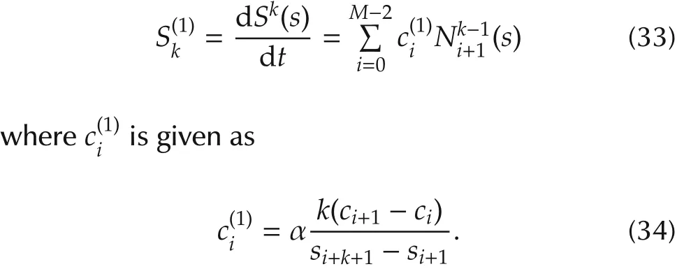
For simplicity,we write equation(34)in a matrix form

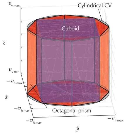
Fig.4 Constrained volume for acceleration.Axis-decoupled methods select an axis-aligned cuboid(the blue cube).The axis-coupled method selects arbitrarily shaped convex polytopes(the octagonal prism).

Following equation(26),there exists an mapping matrix for the control points ofas

Using the results in Section 3.6,one could then construct convex safe regions forAssume the convex region is described by{p∈Rd|Anp?bn},the inequality constraints are Similarly,for non-convex constraints,the time segmentation method can be utilized.

3.8 Input constraints

For a q th order integrator,if its trajectory is represented by an k th order B-spline Sk,then its input is the q th order derivative of Sk.

Therefore,the results in Section 3.7 can be applied to limit the input to the system as equation(39)holds true for arbitrary ordered derivatives.

3.9 Boundary conditions

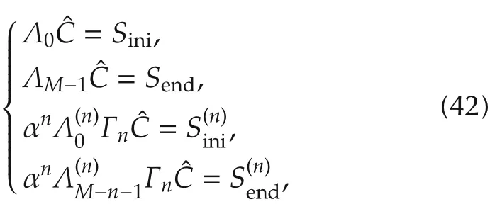
Let Sini,Senddenote the desired initial and final states of the trajectory Sk,respectively.represent the desired initial and final states of the trajectory’s n th derivative,respectively.From Eqs.(1)and(3),the initial and end states of Skare determined by the first and last control points:

From equations(37),(26)and(38),the boundary conditions can be written as

4 Quadratic programming problem

So far,we have formulated convex and quadratic cost functions in equations(9),(11),(25)and(27),and linear constraints in equations(32),(39)and(42).Therefore,it is straightforward to construct a QP to describe the trajectory generation problem as

The QP problem can be solved from various off-the-shelf solvers such as the MATLAB QUADPROG[19]and the IBM CPLEX[20].Among the four types of constraints in Section 1,if the problem only has boundary conditions,then our formulation gives a closed form solution.In robotic applications,the other constraints can usually be omitted through various ad-hoc methods,but the boundary constraints are difficult to be replaced.From equation(42),the elements between the(k+1)th and(M-k)th column of Aeqare all zero when only considering the boundary constraint.To separate out the non-zero parts,we define

and re-arrange the control point matrix C into

Here,the “fixed”part CFis fully determined by the boundary conditions:

In order to isolate the “fixed”part from the optimization problem,we define a mapping matrix Φ:

Then,equation(43)can be written as

By defining

equation(48)can be written as

and equals

and can be further simplified as

Finally,by collecting the terms,there is

5 Flight experiments and analysis

To demonstrate the performance of the proposed approach,real experiments are performed using a small quadrotor as shown in Fig.5.

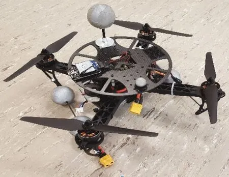
Fig.5 The quadrotor used for experiment.

The quadrotor has been proven as a differential flat system and is commonly approximated as a triple or 4th ordered integrator system during trajectory generation.In this paper,we adopt the 4th order model and also utilize a 4th order B-spline(k=4).The algorithm is implemented in Matlab except when calculating H,where a C application is linked through Mex.Our method is compared to the previous interpolation based trajectory generation for quadrotors[1],[2],the implementation of which is from the open source project[17].

5.1 Point-type data fitting

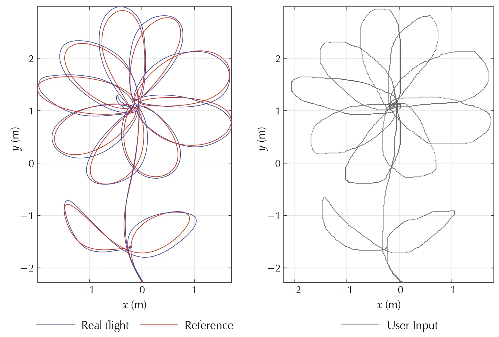
Fig.6 Densely fitting of user sketching inputs.The blue curve shows the real vehicle tracking performance.

In the first example,we demonstrate the algorithm’s capability in fitting point-type nominal plans.The nominal plan is generated through direct user input through drawing.Since the sketching inputs come with a large amount of sampled data points,we formulate the trajectory generation as an approximation problem and achieves better results compared to the previous interpolation based methods[1,2].The major problem with the interpolation based methods is overfitting.Especially in the case of noisy or crudely estimated time-points.The inaccurate time-point would introduce unnecessary excursions.Through ourformulation,the excursions can be reduced by tunning the weighting factors.With the introducing of the deviation cost,the numerical stability of the optimization is also increased.Fig.6 shows the result of fitting a user sketch with more than 1000 data points.The time-points are estimated heuristically with a single integrator model.The proposed method generates a smooth trajectory that could be tracked precisely by the quadrotor while the interpolation method diverges.

5.2 Nominal plan with line-segments

We also compare the performance at fitting a nominal plan consists of line-segments.As mentioned previously,poorly chosen time-points usually lead to large excursions[18].A common practice is to insert intermediate position-points along the line-segments[2].However,it often leads to more aggressive maneuvers of the vehicle.Here,we use the snap cost,which is the integration of the square of the snap along the trajectory,to measure the aggressiveness of the trajectory.

In Fig.7,it shows a comparison between three methods.Methods 1 and 2 are the interpolation based methods using a 7th order polynomial spline.Method 1 only interpolates the original waypoints while Method 2 also inserts and interpolates intermediate position-points.Finally,Method 3 is the proposed technique for fitting line segments.The experiment shows that Methods 2 and 3 perform similarly at fitting the nominal plan with an average deviation of 0.05 m and 0.02 m,respectively.However,compared to Method 2 which gives a snap cost of 6923,Method 3 produces a much less aggressive trajectory with a snap cost of 348.

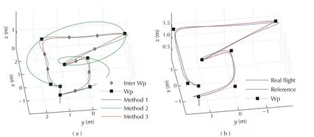
Fig.7 Comparison for fitting line segments.The time-point allocation for the original waypoints are the same for each method.

5.3 Trajectories on desired planes

In a light paint event with quadrotors,it is desirable to have the trajectory stay close to a plane to prevent the shape from distorted when viewed from different angles.We apply the results in Section 3.3.3 to achieve the desired results.In Fig.8,four position-points on the same surface defined an M shaped trajectory.However,if the trajectory now considers the velocity and acceleration constraints,it might cause an asynchronous movement and distort the desired shape,especially when viewed from aside.(see Fig.8(b)).On the other hand,the proposed approach could penalize the deviation to the desired plane and reduce the distortion.

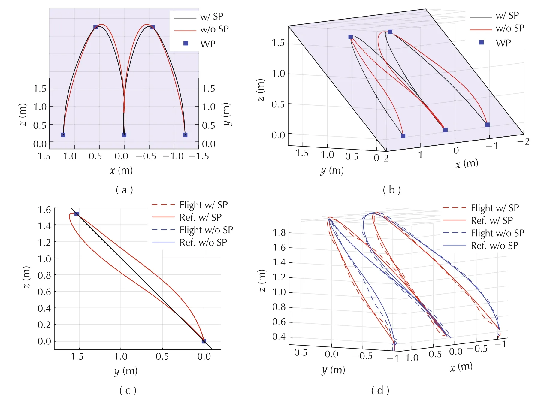
Fig.8 Comparison between trajectory with surface penalty(w/SP)and without surface penalty(w/o SP).(a)0o view.(b)55o view.(c)90o view.(d)Real flight.

5.4 Safety and feasibility

Quadrotors are usually operated in obstacle strewn environments.The safety and feasibility of its trajectory can be guaranteed using the methods presented in Sections 3.6 and 3.7.In Fig.9,the safe operation region is constructed using 7 pieces of oriented bounding boxes.Furthermore,the trajectory is also required to satisfy the following conditions:

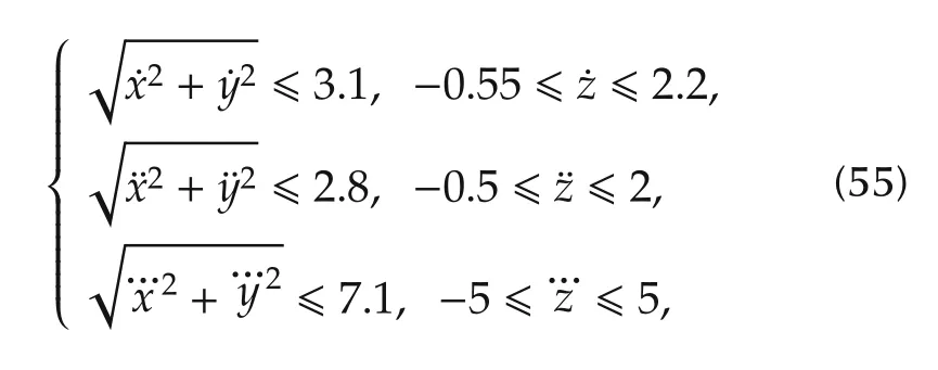
where x,y,z denotes the trajectory’s component on the corresponding axis.These constraints on the velocity,acceleration,and jerk spans three separate cylinders.With the axis-decoupled constraints,the largest axisaligned cuboid is adopted inside the cylinder.Using the proposed axis-coupled constraints,the largest hexagonal prism inside the cylinder is formed.

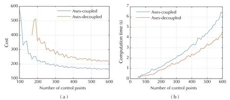
Fig.10 Comparison between axes-coupled and decoupled methods.(a)Cost.(b)Computing time.

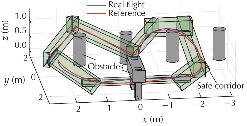
Fig.9 Safe corridor.

We compare the resulting cost value and computational time against the number of control points used(see Fig.10).The formulation with axis-coupled constraints generates trajectories with lower costs but slightly longercomputationaltime.However,italso produces a feasible solution with fewer control points.

6 Conclusions

In this paper,we have presented a method to generate trajectories for chains of integrators using the B-spline technique.It systematically studies the issue of axis-coupling and interval-wise effectiveness.The application includes penalizing the deviation from arbitrary geometric flats.Through the convex hull property,all convex constraints can be satisfied throughoutthe entire trajectory.We have shown that non-convex constraints and nominal plans can be converted into convex ones through time segmentation.To guarantee the real-time capability and reliability which are required in robotic applications,we have formulated the problem into a QP.A closed-form solution has been derived for solving boundary value problems efficiently.Finally,the overall approach has been successfully tested and verified in real experiments using quadrotors which is commonly considered as high-order integrators.