A data-based CR-FPK method for nonlinear structural dynamic systems

Jie Li, Zhongming Jing*

a State Key Laboratory of Disaster Reduction in Civil Engineering, Shanghai 200092, China

b School of Civil Engineering, Tongji University, Shanghai 200092, China

Keywords:Data-driven computational mechanics FPK equation Dimension reduction Cell renormalization Model-free

ABSTRACT Stochastic dynamic analysis of the nonlinear system is an open research question which has drawn many scholars' attention for its importance and challenge. Fokker–Planck–Kolmogorov (FPK)equation is of great significance because of its theoretical strictness and computational accuracy.However, practical difficulties with the FPK method appear when the analysis of multi-degree-offreedom (MDOF) with more general nonlinearity is required. In the present paper, by invoking the idea of equivalence of probability flux, the general high-dimensional FPK equation related to MDOF system is reduced to one-dimensional FPK equation. Then a cell renormalized method(CRM) which is based on the numerical reconstruction of the derived moments of FPK equation is introduced by coarsening the continuous state space into a discretized region of cells. Then the cell renormalized FPK (CR-FPK) equation is solved by difference method. Three numerical examples are illustrated and the effectiveness of proposed method is assessed and verified.

1 Introduction

Stochastic dynamic analysis of nonlinear structure is an open research area which has drawn many scholars' attention for its importance and challenges [1]. In the past decade's considerable effort has been made in developing techniques to calculate the response of nonlinear dynamic systems under random excitation [2, 3].

One of the most broadly applicable procedure to analyze the stochastic dynamic problem is dedicated to the approximation of the underlying equation on the level of probability density function (PDF), i.e. the Liouville, the Fokker–Planck–Kolmogorov (FPK), and the Dostupov–Pugachev equations. Particularly, as a widely investigated equation, FPK equation could govern the transition PDF of a Markov vector process which is constituted by the response of a nonlinear dynamical system to random excitation [4, 5]. However, one major obstacle in solving FPK equations is that they are usually high-dimensional equations where all the state variables should be involved. This produces so challenging problem when high dimensionality and nonlinearity are both involved [2-4]. To circumvent this issue,many approximate procedures are developed for estimating the solution of associated FPK equation [6]. For example, for those nonlinear systems in which the amount of nonlinearity is controlled by a small parameter , the perturbation method is usable by considering the solution as a combination of linear responses and power series of [5]. For Gaussian and some non-Gaussian processes, moment closure method is employed to approximate the solutions FPK equation by assuming that certain higher order moments are neglected or assumed to be related to lower order moments [7]. As a extensively applied and detailed studied method, stochastic averaging method can be applied to a class of procedures in which rapid fluctuations are averaged to provide simpler equations for slowly fluctuating quantities [6, 8,9]. The method of path integration employs a certain interpolation approximation in which the probability density is represented by its values at discrete grid points. This method is first applied by Wehner and Wolfer and aimed at representing probability density by its values at discrete grid point [10]. Then this algorithms is further developed by Crandall [11], Yu et al. [12], and Naess et al. [13]. By exploiting the integrability and resonance property of Hamiltonian dynamics, Huang et al. [6] and Zhu et al. [14] developed an equivalent nonlinear system method to ob-tain the stationary solutions of stochastically excited and dissipated Hamiltonian systems. However, most of the approximation method are limited to stationary solution of lower dimensional FPK equation. For those complex engineering structures, such as high-rise buildings and towers, which exhibit considerable nonlinear property under extreme external loadings such as earthquakes, strong wind, or huge waves, how to solve the corresponding high-dimensional FPK equation is still a prodigiously difficult problem [15, 16]. Nevertheless, when it comes to the point that the deterministic model can hardly be captured, the possibility to embed time-history data directly into the computational models is desirable.

In the present paper, a new numerical method to solve multi-dimensional FPK equation is proposed in which a novel computational method to derive the derivative moments of FPK equation is introduced. The equivalence of the derivative moments of FPK equation in different treatments via the state space description and the random event description is firstly revisited.Then a new dimension reduction approach of the FPK equation of multi-degree-of-freedom (MDOF) nonlinear system is introduced. The idea of cell renormalization is introduced and a reconstruction method is introduced to rebuild the derivative moments of FPK equation. The steps of numerical implementation and additional remarks are outlined. Finally, three numerical examples including a linear single-degree-of-freedom (SDOF) system, an SDOF Duffing oscillator and a 6-DOF nonlinear hysteretic structure are illustrated. The performance of the proposed method is assessed and its results are compared to the result of analytical approach and Monte Carlo simulation (MCS)method. The conclusion and the issues to be further studied are presented in the last part.

2 Equivalent expression of the derivative moment of FPK equation

2.1 Derivation of FPK equation

As well known, there are two procedures of deriving the FPK equation form the nonlinear equation of motion of the dynamic system. The first procedure is commonly seen in groups of physicists and engineers, the drift and diffusion coefficients of FPK equation could be obtained by limit operations applied directly to the equation of motion [17, 18]. In the second procedure,favored by mathematicians, the equations of motion are replaced by the equivalent Itô equations according to certain translation rules. The drift and diffusion coefficients is then obtained by formal operations on the coefficients of the Itô equations [19]. The two procedures are operationally parallel for for non-parametrically excited systems [5].

Consider a general nonlinear SDOF system

where g (·) can be any nonlinear function, ξ (t) is a Gaussian white noise process. As we know, if this nonlinear vibration system can be written as the Itô stochastic differential equation(SDE), its responseis said to be a continuously valued random process with Markov property [20]. Then the following relation exists between the conditional probability functions:

The conditional probability density appearing on the right-hand side of Eq. (2) is especially known as the transition probability density of the Markov process. For an arbitrary continuous random process

if X (t) is Markovian, Eq. (3) reduces to

Equation (4) is known as the Chapman–Kolmogorov–Smoluchowski (CKS) equation, which may be called the compatibility equation for a Markov process [20].

Consider the integral

whereR(y) is an arbitrary function of y which goes to zero sufficiently fast as y approaches + ∞ or - ∞. Specifically, we assume that for any n,

Now Eq. (6) may be written as

The order of the integration and the limit operation is interchangeable as long as the integral converges uniformly in a neighborhood oft. Employing the CKS equation, Eq. (4) goes to

Further assume that the arbitrary functionR(y) can be developed in a Taylor's series about the pointx:

Substituting Eq. (9) into Eq. (8) and integrating first ony,

where

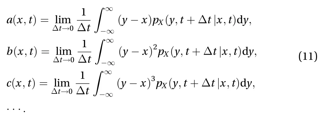
They are called the derivate moments. It is sometimes more indicative to write

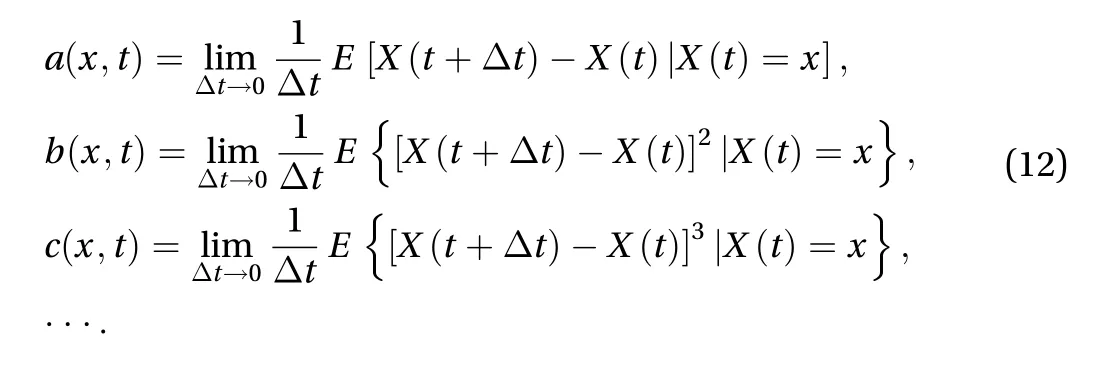
Combining Eqs. (8) and (10) under the consideration of the arbitrariness ofR(x), the following equation can be acquired,

For the dynamic system with Gaussian white noise excitation,the response process would be a diffusion Markov process. For such cases, the higher derivative moment equal zero, then Eq. (13) can be reduced as

in whichpX=p(x,t|x0,t0) is the transition probability density of diffusion Markov process. Equation (14) is the so called FPK forward equation [20].

2.2 Equivalent expression of derivative moments

In general, a stochastic process could be expressed as a stochastic function of a set of independent random parameters.For example, by introducing the stochastic harmonic functions[21], a Gaussian white noise process ξ (t) could be expressed as a function with random variables F (,t). That is

where the ωjand φjare random frequencies and random phase angles, respectively, the amplitudesZ(ωj) are function of ωj, andNis the retained terms of harmonic components. φjare independent uniformly distributed random variables over[0,2].=(ω1, ω2,...,ωs/2,φ1, φ2,...,φs/2)=(Θ1,Θ2,...,Θs)is the involved random vector in thes-dimensional spaces,i.e., p ()=1 for ∈sand otherwise p ()=0, s is the number of the basic random variables.

By doing so, the response of Eq. (1) could be written as a function of random vector. The derivative moments of FPK equation will become

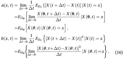
whereEΩXdenote the expectation involves the state space description where all the state variables are involved in the joint PDF, whereas EΩinvolves the random event description where the random source vector is involved together with the physical quantity of concern. Therefore, these equivalent relationship supply a possibility to get an equivalent form of Eq. (14)

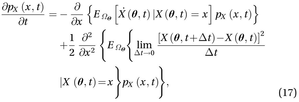
then obtain its numerical solution.

2.3 FPK equation of single–degree-freedom system

In order to give the coherent expression of the FPK equation involves stochastic function description as in Eq. (17), we first examine an SDOF dynamic system with a sort of general form nonlinearity

Due to the property of Gaussian white noise, Eq. (19) is formally equivalent to an Itô SDE

where E[dW(t)]=0 and E{[dW(t)]2}=Ddt. Due to the property of Itô SDE [20], the response of Eq. (18) is Markovian.Therefore, the joint PDF of [X,X˙]T, denoted bypXX˙(x,x˙,t)=pX(,t)is governed by the following FPK forward equation

By limit operations applied to the equation of motion (18) or certain translation to the Itô equation (21), the drift and diffustion coefficients in Eq. (22) could be analytically written as a function of state space vector [22], which inherently admit a equivalent random event description as in Eq. (16)

For the FPK equation of non-parametricly excited SDOF system with an arbitrary nonlinearityg(x,x˙,t) as in Eq. (18), the diffusion coefficientcould be derived by D. The first drift coefficient is predetermined asa1(,t)=x˙. The only coefficient function need to be estimated is a2(,t) in order to get the solution of FPK Eq. (22).

3 MDOF nonlinear system under random excitation

For practical MDOF system, the dimension of the FPK equation is often too high to get a satisfactory result whether in analytical ways or numerical ways. By invoking the equicalent between the space description and random event description,the high-dimensional FPK equation could be reduced into a lower one in term of the quantity of our interest.

3.1 MDOF nonlinear system under random excitation

Consider the equation of motion of a nonlinear MDOF system:

where is thendby one displacement vector, the overdo denotes time derivative,g(·) can be any nonlinear vector function, (t) is thend-dimensional Gaussian white noise stochastic excitation vector with E[(t)]= and E[(t)T(t+τ)]=δ(τ), in which is ndby ndpositive definite diagonal matrix.

Introducing state vector,

Equation (24) could be rewritten as

where is the basic random vector involved in the system when the random excitation vector¯(t) is truncated in frequency domain and represented by ¯ (t)=¯(,t).

In this case, Eq. (27) could be understood as an Itô SDE. Thus the joint PDF of (t),p(,t) is governed by a corresponding 2ndFPK equation [20, 23]:

The derivative momentsai(,t) andbij(,t) in Eq. (28) could be analytically achieved as:

For most engineering problems, solving the partial differential Eq. (28) is unpractical whennd≥2, either by analytical or numerical methods. Hence, a reduced lower dimension of FPK equation is needed.

3.2 Dimension reduction of FPK equation

Generally, to capture the probabilistic information of some of the state entities of concern, rather than the joint PDF of the whole augmented state vector, it is possible to marginalize the original FPK equation in terms of those state entities not to be concerned [24].

In order to do so, we can introduce the idea of probability fluxes

If only the probabilistic information ofl(1≤l≤2nd) is of concern and the solution of this concerned quantity is existent,unique and must depend on the parameter vector , define

Likewise, the acceleration of Ylgives

Marginalize Eq. (28) in terms ofy1,y2,...,y2ndexcludingyland ynd+l, will yield

Obviously, the first probability fluxcan be rewritten as

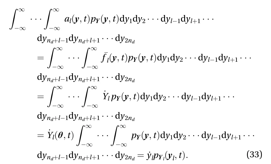
As regards the second probability fluxnote that if the equivalent relationship as in Eq. (23) is invoked as

We immediately have

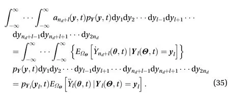
Here the equalityYnd+l=in Eq. (25) is used.

Let

Hence the FPK Eq. (32) could be transformed as

Therefore, the problem of tackling Eq. (28) is transformed into constructing the derivative momentwhich is the only undetermined coefficient in the corresponding dimension reduced FPK Eq. (37).

4 Cell renormalized FPK equation

In the previous sections, the dimension of FPK equation is reduced into Eq. (37) by the equivalence property of two descriptions. Then the stochastic analysis of general MDOF system(24) could be settled by Eq. (37). However, there are difficulties in numerically building the derivative momentAlin Eq. (37). As previously shown, the conditional expectation of acceleration given an eventis involved in calculatingAl. However,the numerical integration in Eq. (36) cannot be simply calculated by Crude Monte Carlo method because Al(l,t) us a function ofandy˙l. To overcome this issue, we employ a new method called Cell Renormalized method to numerically acquire the derivative moment Aland the corresponding cell renormalized FPK (CR-FPK) equation which is relevant to the state vector of our interest.

4.1 Cell renormalized method

To calculate the derivative moment numerically and construct the corresponding dimension-reduced partial differential equation which gives the model-free characterization of nonlinear stochastic system, we introduce a cell approaching method in this paper. The first step in the method is to coarsen the continuous state space [x(l),x(u))×[x(l),x(u)) under consideration into a discretized region of cells, where x(l)and x(u), i=1,2 in dicate the lower and upper limits of the state space. Each cell is uniquely identified by(j)=[,],z ∈ Z,j=1,2,···,M,is the total number of cells. The cell spacingh1,h2is consistent in each dimension such that for each cell centered at

The concerned region which is described by

The corresponding two-dimensional subset S of cell state space is defined as

Figure 1 shows an example in a continuous state spacewith.

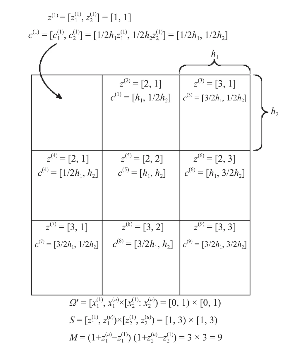
Fig. 1. Example of generalized cell mapping in [ 0,1)×[0,1).

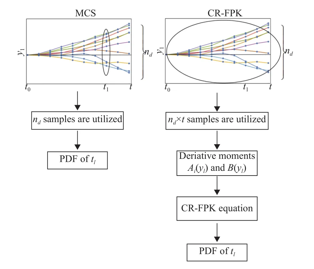
Fig. 2. Difference of flowchart between MCS and CR-FPK.

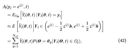
in which P (=q|l∈ Ωj) is a conditional probability.

Normally, we cannot directly get the probability P(=q|l(,t)∈Ωj)because the inherent correlation information between random events =qandl(,t)∈ Ωjare unclear. However, by introducing the Bayes' rule, this probability can be decomposed as:

where P (l∈ Ωj|=q) in the numerator of Eq. (38) is the probability of observing eventl∈ Ωjgiven thatis true,that is

Introducing cell renormalized assigned probability

Then from Eqs. (43) to (46), Eq. (42) will be changed to

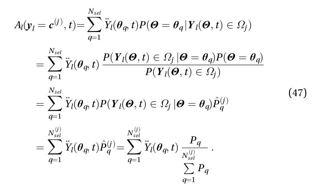
In the derivation of achieving Eq. (47), we can clearly see the process of transforming general assigned probabilityinto aset of normalized assigned probability in each cell. This is why the proposed method is called "cell renormalized" FPK method in this paper.

4.2 Numerical implementation of CR-FPK

As described before, through constructing the dimension reduced FPK equation, CR-FPK method is capable of dealing with MDOF system with general nonlinearity and randomness. The first step of CR-FPK method is to evaluate the derivative moment due to the drift by Eq. (47). Then, the obtained dimension reduced partial differential equation, which is called CR-FPK equation in this paper, could gives a model-free characterization of nonlinear stochastic system. After numerically solve the equation by finite difference method, the numerical value ofwill be finally yield.

The procedures of CR-FPK method are described as follows:Step 1: Specify the representative point setNsel}and the corresponding assigned probabilitiesPq,q=1,2,···,Nselin the domain . The detail of this step could be found in Appendix A [23, 25-27].

Step 2: For each =q, solve the embedded dynamics Eq. (27)to yield

Step 3: Apply the cell renormalized method discussed in Sect. 4.1 and 4.2 and transform the continuous state space into a discretized cell space. Substitute thin Eq. (47) to get the discrete values of derivative moment in cell space. Then utilize the discrete values of derivative momentAl((j),t)as train data to build a regression model of derivative moment(l,t).

Step 4: Substitute the obtained numerical estimated derivative moments in Eq. and solve it by the finite difference method, say,the Crank–Nicolson scheme. This will finally yield the transient PDF.

5 Numerical Examples

5.1 Random vibration of a linear SDOF system

First, a simple SDOF system subjected to Gaussian white noise is considered to testify the effectiveness of the proposed method for linear system

where c0is the damping coefficient, k0is the stiffness coefficient,ξ0(t)is a unit white noise with E[ξ0(t)]=0 andE[ξ0(t)ξ0(t+ τ)]=D0δ(τ). The corresponding analytical FPK equation governing the instantaneous joint PDF of[X˙(t),X(t)]Tgives

In this example, the FPK equation is a two dimensional partial differential equation which can be solved by various numerical methods. Although the analytical FPK equation and the corresponding analytical derivative moments are obtainable in this example, the proposed method could be taken to verify its effectiveness by comparing the results of CR-FPK equation with the numerical result of analytical FPK equation. Obviously, the major sources of the calculation error are the difference between the analytical derivative moment c0x˙+k0x and the numerically constructed derivative moment,t) and the imperfection of white noise simulation. For this purpose, we are going to analyses the difference between theoretical derivative momentand constructed derivative moment(,t), then calculate the joint probability distribution pX˙X(x˙,x) and marginal probability distributionsandpX˙(x˙) at typical time instants by both method.

In the numerical study, we takeD0=1,c0=2.3, andThe upper cut-off frequency of the white noise israd/s. Inthe analysis,200 representativepointsgenerated by generalized F (GF)-discrepancy are adopted and 200 deterministic representative time-histories data are embedded.Suppose for the sake of simplicity that the derivative moment needs to be estimated is time-invariant, i.e., only a function of variablesand. Then we can utilize the representative data over the entire time period to estimate the derivative moment which can be reduced as. And the utilization of information can be more efficient than directly Monte Carlo, as shown in Fig. 2. Considering the number of calls to deterministic model isand the time step and duration of time history are ΔtandTrespectively. The conventional MCS method can only utilizeNselsamples to estimate a instantaneous PDF and the small sample problem can cause fluctuation at the tail of PDF. However, the proposed method can make full use of all samplesand hence improve the tail of PDF.

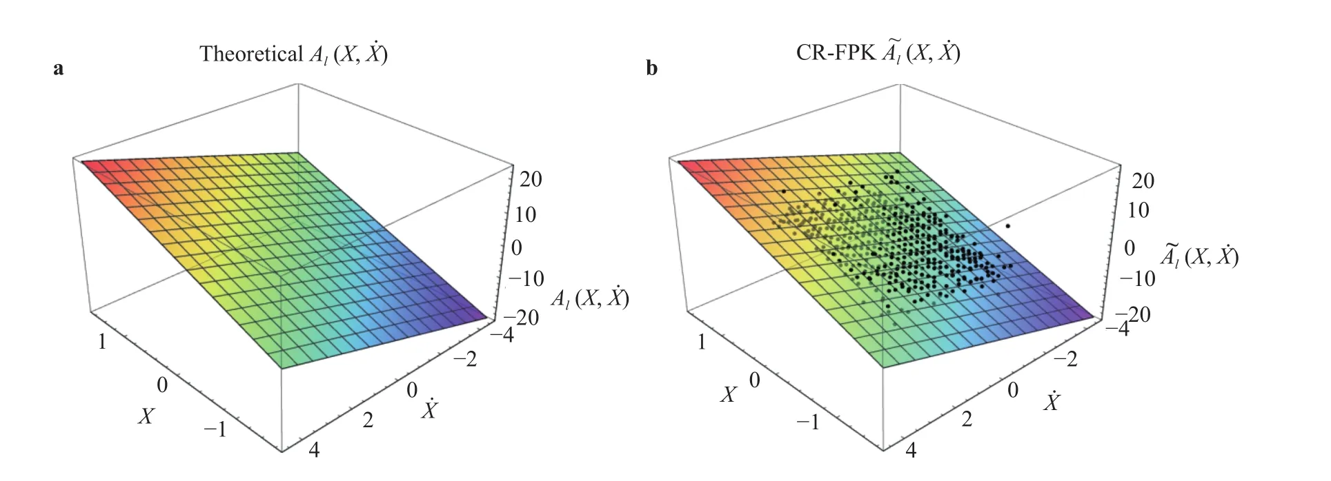
Fig. 3. Comparison of derivative moment by different method (Example 1). a Analytical derivative moment A l(x,x˙)=7.8x+2.3x˙, b derivative moment of CR-FPK A~ l(x,x˙)=7.743x+2.281x˙.

Fig. 4. PDFs of responses at different time instants (Example 1). a Displacement, b velocity.

Fig. 5. Time-varying variance of responses (Example 1). a Displacement, b velocity.

The cell size adopted here is 3 2×32=1024 regular cells to cover [ -1.6,1.6)×[-4.6,4.6). By using first order polynomial regression model to fit the discrete values of derivative momentAl((j)), the resulting derivative moment is7.743x+2.281x˙. Figure 3 shows the 3D plots of the analytical derivative momentk0x and the estimated derivative moment A~l(x,x˙). In all subfigures, the black dots indicate the calculated discrete values ofAl((j)). It is seen that the derivative moment obtained by theoretical method and the proposed method(labeled as CR-FPK) are close to each other. To offer a direct verification and evaluation of the effectiveness of the proposed method, the marginal PDFs ofandare calculated through numerical integration. Form Fig. 4 it is seen that the result of the proposed method exhibits good numerical accuracy within the limited number of calls to model. The same conclusion can also be drawn in Fig. 5, which shows the time-varying variance of responses.

5.2 Random vibration of a Duffing oscillator

Consider a Duffing oscillator subjected to Gaussian white noise

where γ is the damping coefficient, ε is a coefficient characterizing the degree of nonlinearity, ξ (t) is a white noise with E [ξ(t)]=0 and E [ξ(t)ξ(t+ τ)]=Dδ(τ). When Eq. (50) is understood as an Itô SDE, the analytical FPK equation governing the instantaneous joint PDF of [X˙(t),X(t)]Texists as

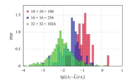
Fig. 6. Histograms of the log of the relative error in the estimating of derivative moment.

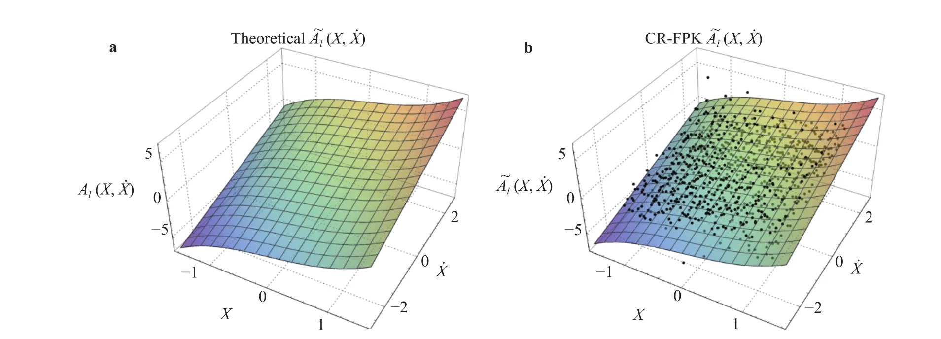
Fig. 7. Comparison of derivative moment by different method (Example 2). a Analytical derivative moment =x+0.5x3+x˙, b derivative moment of CR-FPK (x,x˙)=1.090x+0.512x3+1.093x˙.

and the stationary solution is given by [28]

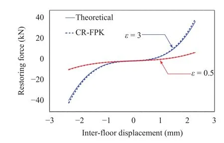
Fig. 8. Estimated restoring force for weak and strong nonlinearity.

where C1is a normalization constant. The stationary marginal PDF ofX(t) andcould be acquired through numerical integration expediently. In this numerical study, we take γ =1,ε=0.5, and D =2. The upper cut-off frequency of the white noise is ωu=100 rad/s. The number of adopted representative points and the corresponding derived representative timehistories 300 in the example.

There are three different configurations of cell sizes are studied in this example. The cell sizes are taken to be 1 0×10=100,16×16=256, and 32×32=1024 regular cells to cover[-2.7,2.7)×[-4.0,4.0). Figure 6 is the histograms of logarithm error between the calculated derivative moments and the theoretical derivative moments in Eq. (51). The result shows that the numerical error in estimating derivative moment is decreasing with the increase of refinement of cell sizes. Thus, the relatively high level refinement using a cell size 3 2×32=1024 was adopted in the next calculations.

We use third order polynomial regression model to fit the discrete values of derivative momentAl((j)), the resulting derivative moment is,=1.090x+0.512x3+1.093x˙. Figure 7 shows the 3D plots of the analytical derivative moment+(x+εx3)and the estimated derivative momentA~l(x,x˙). It is seen that derivative moments obtained by theoretical method and the proposed method are visually identical. To tesify the effectiveness of the proposed method for both weak and strong nonlinearity cases, CR-FPK method for different parameter set-tings (and ε =3) are studied and their results of estimated restoring forcef(X)=(1+εX2)Xare shown in Fig. 8.Form the figure we can see that, unlike some conventional method such as perturbation method, the CR-FPK method is free of strong nonlinearity problem and exhibits good accuracy whether the nonlinearity being weak or strong.

Fig. 9. PDFs of responses at different time instants (Example 2). a Displacement, b velocity.

Fig. 10. Time-varying variance of responses (Example 2). a Displacement, b velocity.

Fig. 11. PDFs of responses at 10 s. a Displacement, b velocity.

Same as in Example 1, to justify the effectiveness of the proposed method for the nonlinear system, the derivative moments of analytical 2-dimensional FPK equation and CR-FPK equation,the joint probability distribution pX˙X(), marginal probability distributionspX(x) andat typical time instants and timevarying variance of responses are all investigated. In Figs. 9 and 10 shown are the marginal PDF ofX(t) andat typical time instants and the time-varying variance of responses. Form these figures it is seen that the result of the proposed method fits well with the result of theoretical FPK. According to the analytical stationary solution, the proposed method shows superior accuracy in Figs. 11 and 12 compare with crude MCS with 300 trials, which is the exact same number of trials adopted in CR-FPK method.The logarithmic coordinate system in Fig. 12 exhibits the higheraccuracy of the proposed method more clearly, especially at the tails of the distribution. In Table 1, Kullback–Leibler (K-L) information distance is introduced as a quantitative index to evaluate the difference between two probability distribution functions, which draws the same conclusion as the previous qualitative results.

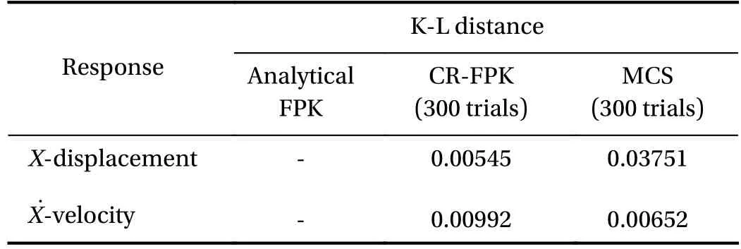
Table 1 Comparison of K-L distance between PDFs of CR-FPK method, analytical FPK equation and MCS (Example 2)

Fig. 12. PDFs of responses at 10 s in logarithmic coordinate system. a Displacement, b velocity.

5.3 A 6-DOF nonlinear hysteretic structure

Consider a 6-story floor-shear structure shown in Fig. 13. The lumped masses of every floor are 3.9, 3.5, 3.2, 2.8, 2.4, 2.1 (×105kg), respectively. The height of each floor is h = 2.5 m. The Rayleigh damping is adopted aswhereIn the simulation of the nonlinear restoring force of structure, the Bouc–Wen model is introduced as [29]:

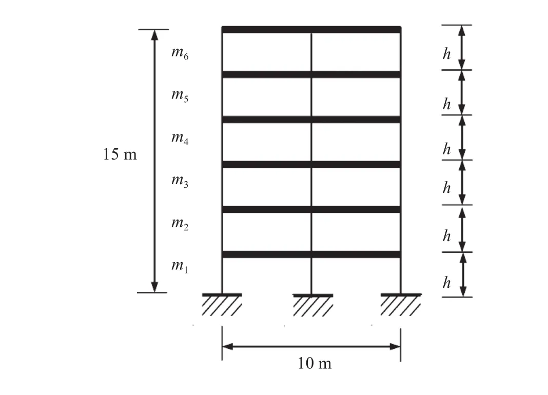
Fig. 13. The 6-story structure.

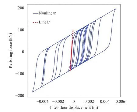
Fig. 14. A typical picture of restoring force vs. inter-story displacement.

Fig. 15. PDFs of top responses at different time instants. a Displacement, b velocity.

Fig. 16. CDFs of responses in the linear coordinate system. a Displacement, b velocity.

Fig. 17. CDFs of responses in the logarithmic coordinate system. a Displacement, b velocity.

Table 2 Comparison of K-L distance between PDFs of CR-FPK method, 10000 trials of MCS and 1000 trials of MCS (Example 3)

The character of the restoring force is defined by 6 parameters, which are, and. The typical restoring force versus inter-story is shown in Fig. 14 which indicates a strong nonlinearity compare to the linear counterpart. From this figure, the typical hysteretic property is observed so that a strong nonlinearity is inherent in the structure.

In this case, again the GF-discrepancy method is adopted and 1000 representative time-histories data are generated. Extra 10000 trails are carried out for MCS whose result can be treated as a benchmark. The cells of size 3 2×32 are taken to cover the state space region [- 0.015,0.015)×[-0.03,0.03).

Not like the first two examples, in this case the derivative moment needs to be calculated is a function of time, i.e.,cannot be simplified as. Therefore, the whole 5 s time period is divided into five periods including 0–0.5 s, 0.5–1.0 s,1.0–1.5 s, 1.5–2.0 s, and 2.0–2.5 s. The derivative moment in each time period could be considered as a function which is irrelevant to time. Then we can use a third order polynomial model to fit the discrete values ofat each time period. In Fig. 15 shown are the PDFs of the top displacement and velocity at different time instants, 1.5 s, 2.0 s, and 2.5 s. As shown in Fig. 15a, b, the global property of PDFs obtained by the 10000 trials of MCS and the proposed method is close to each other. The cumulative distribution functions (CDFs), obtained by the 10000 trials of MCS, by the proposed method with 1000 trials of simulation and by 1000 trails of MCS are shown in Figs. 16 and 17 in an ordinary coordinate system and logarithmic coordinate system,respectively. It is observed form Fig. 16 that both MCS and the proposed method (CR-FPK) accord quite well with the CDF by 10000 trials of MCS. However, form Fig. 17 it is seen that the proposed method has higher accuracy than MCS with the same number of simulation, particularly at the tails of the distribution.The K-L distance information in Table 2 also draws the similar conclusion as in the figures.

The examples here demonstrate the feasibility of the proposed approach, the further studies about the numerical errors induced by the frequency band truncation of white noise and the embedded numerical algorithm of FPK equation are still to be done. Besides, the possible adoption of other numerical method for low-dimensional FPK equations, e.g., the path integral method, is also of great interest.

Acknowledgements:

This research is financially supported by the National Natural Science Foundation of China (Grants 91315301 and 51261120374).

Appendix A: Determination of the representative point sets

A high-dimensional numerical integral in domaincan be rewritten as weighted form

where gqrefers to the weights satisfying

qis an sdimensional uniform point set, andnis the number of discretized points. The uniformity of the point setcan be measured by the star discrepancy[30]

In Eq. (55),N(Mn[0,)) denotes the number of points scattered in the s-dimensional hyper-rectangledenotes the volume of the s-dimensional hyper-rectangle. The largest error in the numerical integration of Eq. (54) can be estimated by the Koksma–Hlawka inequality:

where TV(f) is the total variation of the function f, which characterizes the degree of irregularity of f (). For non-uniform distributions, the star discrepancy is extended to the F-discrepancy:

whereF() is the joint CDF of the random vector=(X1,X2,...,Xs), andFn() is the empirical CDF:

whereI(·) is the indicator function, andI(A)=1 if and only ifAholds true, otherwiseI(A)=0.

Instead of using equal weights, 1/n, assigned probabilities,which correspond to the unequal weights in Eq. (54), are required to be calculated first. The representative volume is first defined as the Voronoi cell:

Using this definition, the empirical CDF defined in Eq. (58) is modified as:

wherepqis the assigned probability.

The extended F-discrepancyDEF(Mn) (EF-discrepancy) derived from Eqs. (55) and (57) can be used to indicate the performance of the point set. A small EF-discrepancy is indicative of better numerical accuracy. However, direct computation of the EF-discrepancy for high-dimensional problems is an NP-hard problem, which is intractable in practical applications. To avoid this difficulty, the GF-discrepancy is proposed as:

whereFi(x) is the marginal CDF of thei-th random variableXi,andFn,i(x) is the empirical marginal CDF involving the effects of assigned probabilities in Eq. (60). For most practical problems with bounded total variation, a small GF-discrepancy in a point set usually leads to higher accuracy.

Therefore, the procedure for determining the representative point sets can be divided into two steps: first, an initial point set such as a Sobol sequence is generated, and then the point set is rearranged by reducing the GF-discrepancy. To obtain a representative point set with small GF-discrepancy,ninitial pointsq=(xq,1,xq,2,...,xq,s), whereq=1,2,...,nare first generated from a Sobol setIn={q=(uq,1,uq,2,...,uq,s),q=1,2,...,n}over a unit hypercube using

After the assigned-probabilities pqof the n pointswhere q=1,2,...,n, are evaluated according to the Voronoi cell in Eq. (59), a similar transformation is performed to reduce the GF-discrepancy: