Adaptive sliding mode control for limit protection of aircraft engines
2018-07-24ShuboYANGXiWANGBeiYANG
Shubo YANG,Xi WANG,*,Bei YANG
aCollaborative Innovation Center for Advanced Aero-Engine,Beihang University,Beijing 100083,China
bSchool of Energy and Power Engineering,Beihang University,Beijing 100083,China
KEYWORDS Adaptive control;Aircraft engine;Estimators;Protection;Sliding mode control
Abstract In practice,some sensors of aircraft engines naturally fail to obtain an acceptable measurement for control propose,which will severely degrade the system performance and even deactivate the limit protection function.This paper proposes an adaptive strategy for the limit protection task under unreliable measurement.With the help of a nominal system,an online estimator with gradient adaption law and low-passfilter is devised to evaluate output uncertainty.Based on the estimation result,a sliding mode controller is designed by defining a sliding surface and deriving a control law.Using Lyapunov theorem,the stability of the online estimator and the closed-loop system is detailedly proven.Simulations based on a reliable turbofan model are presented,which verify the stability and effectiveness of the proposed method.Simulation results show that the online estimator can operate against the measurement noise,and the sliding controller can keep relevant outputs within their limits despite slow-response sensors.
1.Introduction
This paper is concerned with the problem of limit protection under unreliable measurement,relevant to practical situations where system outputs are difficult to be measured but should be kept within safe boundary.This situation arises,for instance,in aircraft engine control,where outputs such as turbinetemperatureand compressorpressuremustbe regulated within limits,while the corresponding sensors suffer considerable uncertainties.
Limit protection,which frequently exists as an auxiliary part in control systems,is absolutely not the primary intention of control but is a necessary guarantee of safety.As in the case of aircraft engine control,the main objective is to provide the desired thrust based on the position of the throttle,nevertheless,limit protection is indispensable to keep the engine operating within the limits.1,2Fig.1 shows the widely used architecture of a typical system in aircraft engine control field,which contains steady-state control(primary control),transient control and limit protection.Despite multi-regulator,only the selected control input is available to handle all those three functions.The specific meanings of variables in Fig.1 can be found in Ref.3.

Fig.1 Typical architecture in aircraft engine control field.3
There are plenty of candidates that can be applied to design the regulators for limit protection.Proportional-Integral-Deri vative(PID)control with gain-scheduling technique has been used for decades in the aerospace industry.4–8Sliding Mode Control(SMC)is well-known with mature theories and numerous successful applications.9,10With the one-sided convergence property,SMC is especially suitable for limit protection tasks.In the case of aircraft engine control,SMC regulators have been developed to supplant traditional linear regulators,where SMC can strictly keep relevant outputs within their limits and improve the control performance.3,11–13
In aircraft engine control field,various kinds of sensors are applied to measure rotor speed,temperature and pressure.Therefore,a universal assumption is made in most studies that the states and outputs of a turbo-plant are measurable.In practical situations,however,some sensors naturally failed to obtain the accurate parameters immediately.Because of the need to shield the thermocouples,for example,the temperature measurement has slow response time and is not particularly good for control proposes.2This motivates a reconsideration of the uncertainties in measurement.
For the control tasks with parameter uncertainty,adaptive control is useful to improve control performance online by an adaptation or estimation mechanism.Generally,there are two main approaches for adaptive control.One is the so-called Model-Reference Adaptive Control(MRAC),and the other is the so-called self-turning control.In the former approach,a reference model is introduced for the adaption of unknown parameters,14–16while in the latter approach,an estimator is designed to judge the unknown parameters.Unlike in MRAC design where the parameter adaption law is affected by the choice of the control law,the estimation law is independent of the choice of control law in self-turning control.17
In this article,we concentrate on the limit protection task,which is a sub-problem in the entire control system.Accordingly,an adaptive sliding mode regulator is proposed with system uncertainties considered,especially the ones in output measurement.The rest of this paper is organized as follows:First,a tracking problem with system uncertaintiesis described.Next,an online estimator and its adaptive law are devised to judge the output uncertainties and remedy their adverse effects on output measurements.Then,a sliding controller coupled with the estimator is designed by defining a sliding surface and deriving a SMC law.The system stability on sliding surface is detailedly proven and the reachability of sliding surface is guaranteed.And then,simulations based on a reliable nonlinear turbofan plant are presented,which verify the effectiveness of the proposed controller.Finally,we conclude the paper.
2.Problem formulation
Consider the uncertain dynamical system

where x(t)∈ Rnis the measurable state vector,u(t)∈ Rmis the control input and y(t)∈Rmis the output vector;A,B,C,D are constant matrices of appropriate dimensions;ΔA(t)and ΔB(t)represent the state and the input uncertainty respectively;f(t)represent the output uncertainty.With a desired signal r(t)∈Rmgiven,we intend to devise a feedback control so that the output y(t)tracks r(t)as time goes to infinity.
The following assumption of ΔA(t)and ΔB(t)is made.
Assumption 1.The uncertainty matrix ΔA(t)and ΔB(t)satisfy

where E,Haand Hbare known constant matrices,while Fa(t)and Fb(t)are unknown time-varying matricessatisfying FaT(t)Fa(t)≤I and FbT(t)Fb(t)≤I.
Due to an unknown f(t),y(t)cannot be acquired by the known states and inputs,which makes it elusive to achieve the tracking problem.However,the desire to obtain an available y(t)motivates us to design an online estimator in the next section.
3.Online estimator design
To provide an accurate estimation of f(t),we utilize both output measurements and the nominal system of Eq.(1).
As mentioned before,sensors for output measurement y(t),temperature for instance,are unacceptable due to slow response time.We regard them as first-order dynamics for convenience with the following form:

where ys(t)∈ Rmis the output vector of sensors and τiis the time constant of theith sensor.
The nominal system of Eq.(1)can be written as

Substituting Eq.(4)into Eq.(1)yields

It is noted that y(t)in Eq.(5)has been decomposed into a reference y*(t)and the difference between y(t)and y*(t).Substituting Eq.(5)into Eq.(3)yields

To estimate unknown parameters,we firstly need an estimation model to relate the available data to the unknown parameters.Model in Eq.(6)can be used for estimation seemingly;however,the derivative of ys(t)is undesirable due to measurement noise.It is necessary to adopt afilter to eliminate the derivative of ys(t)in Eq.(6).Filtering both sides of Eq.(6)by(sI+ Λf)-1,wheresis the Laplace operator and Λf=diag(λ1,λ2,...,λm)is am-dimensional diagonal matrix with known positive constant parameters,leads to the form

Relating to unknown f(t)directly,a(t)is the parameter to be estimated.According to Eq.(5),we know that a(t)indicates the difference between y(t)and y*(t).Assuming that the dynamic of real system is approximately similar to that of the nominal system,we can regard the difference a(t)as a slowly-varying parameter.
The estimation of a(t)is

One can predict the value of Y(t)based on the estimation of a(t)and the model Eq.(7)

The difference between the predicted output and the measured output Y(t)is called the prediction error,denoted by e(t)where(t)=(t)-a(t)is the parameter estimation error.

To estimate the unknown parameters,we apply a technique known as ‘gradient estimation”.17–19With the update law

wherep0is a positive number called the estimator gain,the following theory will show the convergence of the estimation.
Theorem 117.Consider the estimation model in Eq.(7)and the estimation error in Eq.(11).If the estimation law is adopted as Eq.(12),the estimator is globally asymptotically stable and(t)→ 0 ast→ ∞.
Proof.Consider the Lyapunov candidate

Its derivative is easily found to be

It is noted that the derivative ofV1(t)equals 0 if and only if the estimation error(t)is 0.Hence,the estimator is globally asymptotically stable and(t)→ 0 ast→ ∞.
According to the estimation of a(t),the estimation of f(t)will be easily obtained by Eq.(9).□
4.Controller design
Oncefinishing the online estimator,we next move to the choice of control law.With the estimation of f(t),unknown y(t)can be replaced by its estimation to achieve the original tracking problem.

Consider the sliding function

Combining Eqs.(15)and(16)yields

Assumption 2.The estimation of f(t)can be considered as

Then we consider the property of system Eq.(1)in sliding mode.On the sliding surface S(t)=0,the equivalent control input can be written as

Substituting Eq.(19)into Eq.(1)yields

where N(t)=ΔA(t)-(B+ΔB(t))(D+ΔD(t))-1(C+ΔC(t)),M(t)=(B+ΔB(t))(D+ΔD(t))-1.Asiswell-known,the stability of a linear inhomogeneous equation equals that of the corresponding homogeneous equation.Therefore,we only discuss the stability of Eq.(20)with r(t)=0.
Lemma 1(Bellman20).If c0≥0,p:R+→R+andq:R+→R+are integrable,and if

then

Theorem 220,21.Consider the linear system

Suppose that for somec1,c2≥0

If there exists a positive σ satisfying

system Eq.(23)is marginally stable.
Proof.Every solution of Eq.(23)satisfies a linear integral equation

Using Eq.(24)and Eq.(25),and multiplying ec2ton each side,

Applying Lemma 1,we have

According to Eq.(25),(σ-c2/c1)is strictly negative,and we can conclude that system Eq.(23)is marginally stable.
After obtaining the sliding function,we next design the sliding control law to attract the system trajectory tending to S(t)=0 infinite time.According to the velocity form,we control the system via integrated inputs,rather than inputs themselves.Therefore,the control law for system Eq.(1)is synthesized as

where ξ > 1,and

In the sequel,it will be shown that the SMC law Eq.(30)can globally drive the system state trajectories onto the sliding surface. □
Theorem 3.Consider the system Eq.(1)with Assumption 1 and the sliding surface Eq.(16)where r(t)is a constant.If the SMC law is synthesized as Eq.(30),it is then shown that the system state trajectories can be globally attracted onto the sliding surface S(t)=0.
Proof.Choose the Lyapunov function

By utilizing Eq.(1),the derivative ofV2(t)can be written as

This means that the reachability of the sliding surface Eq.(16)can be guaranteed by the SMC law Eq.(30).□
5.Turbofan engine example
We apply the proposed adaptive sliding regulator to a turbofan modelofthe GeneralElectric CF6 series.The component-based model is implemented using MATLAB and with the aid of Simulink Toolbox for the Modeling and Analysis of Thermodynamic Systems(T-MATS),which is an open source thermodynamic modeling package initialed on behalf of NASA.22All the engine performance maps and relevant data are acquired from Gas turbine Simulation Program(GSP).23This engine model,which has been also used in other closed-loop control research,24,25is the basis of subsequent controller design and closed-loop simulations.
Without loss of generality,we simulate the case of temperature limit protection with the above model,where the plant has two states(shaft speed of two rotors),a single input(mass fuel flow)and a single output(exhaust gas temperature).Note that all the variables have been normalized by their design values:x1(t)=N1(t)/N1,desis the normalized fan speed,andN1,des=3390 r/min is the design value;x2(t)=N2(t)/N2,desis the normalized high pressure spool speed,andN2,des=10300 r/min is the design value;u(t)=Wf(t)/Wf,desis the normalized fuel flow control input,andWf,des=2.4912 kg/s is the design value;in addition,y(t)=T45(t)/T45,desis the normalized exhaust gas temperature,andT45,des=1084 K is the design value.It is noted that since we choose a single-input single-output system as our example,i.e.m=1,allmdimension vectors are simplified to scalars like e(t),f(t),S(t),etc.
Under the standard day sea level condition,we select the design point(x1=1,x2=1)as a benchmark where the linearization matrices can be obtained as follows:

5.1.Simulation of online estimator
Before verifying the proposed adaptive sliding regulator,we intend to show the performance of the online estimator.A test platform is depicted as Fig.2.
In Fig.2,the engine operates with a given input u(t),while a sensor is applied to measure the unknown y(t).ys(t)is the measurement result with slow response and noise(the magnitude of noise is less than 0.1).Utilizing ys(t),input u(t)and measurable states x(t),our online estimator will obtain the estimation of y(t).To show the necessity of filtering,an alternative estimator is provided as reference.
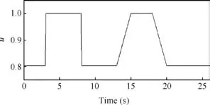
Other simulation parameters are τ1=1,λ1=4,andp0=400.With a step and slope input given in Fig.3,simulation results are shown in Fig.4 and Fig.5.
Fig.4 shows the history of estimation result,where the only difference is whether measurement noise is introduced.T45andT45-sensordenote real and measured temperature respectively.T45-estimator1is the temperature modified by the proposed adaptive estimator andT45-estimator2is that modified by simple lead correction.In Fig.4(a),measuredT45has a slow response obviously,and both estimators operate with acceptable performance according to the realT45.In Fig.4(b),the estimator without filtering is considerably disturbed by measurement noise;however,the proposed online estimator still calculate an acceptable estimation.
Fig.5showstheevolutionofthepredictionerror.Thesteadystate error is always zero,which complies with Theorem 1.
5.2.Simulation of limit protection
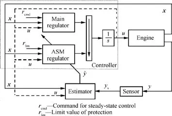
With the aid of the online estimator,the proposed adaptive sliding regulator is implemented.In order to verify the protection function,the main regulator is also required.A reliable regulator is introduced for steady-state control.25An overview of the system structure is shown in Fig.6.
With other parameters as follows:

we simulate the engine acceleration fromN1=1898 r/min(56%ofN1,des)to take off condition under the standard day sea level condition.Simulation results are shown in Fig.7 to Fig.21.
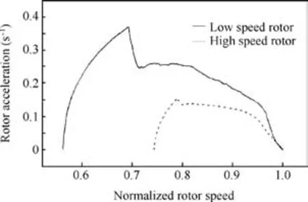
Fig.7 shows the histories of the nonlinear system states x(t).We can conclude that the normalized fan speedx1(t)tracks the reference signal properly.Fig.8 shows the phase plot for both rotor dynamics.

Fig.2 Estimator test platform.
Fig.9 shows the history of exhaust gas temperatureT45.T45-sensor,the output of a sensor model,has a slow response and is far within the limit boundary.T45-estimator,the result of our online estimation,tracks and does not exceed the limit line when the protection is active.However,due to the estimation error in transient process,the realT45differs fromT45-estimatorslightly.

Fig.3 Normalized fuel flow.

Fig.4 Normalized temperature.

Fig.5 Prediction error.

Fig.6 Overview of system structure.
Fig.10 shows the normalized fuel flow histories as the control input to the plant.Fig.11 shows the fuel flow rate of the two regulators and the selection result.As can be observed in Figs.10 and 11,the regulator for limit protection is active during the last half of the acceleration.
To verify that Assumption 1 is satisfied,we use online linearization technique to evaluate the uncertainties.Figs.12 and 13 show state uncertainty ΔA(t)and input uncertainty ΔB(t)separately.The elements of ΔA(t)2×2are Δa11(t),Δa12(t), Δa21(t)and Δa22(t)while the elements of ΔB(t)2×1are Δb1(t)and Δb2(t).With the specific E,Haand Hbin Eq.(35),Fig.14 shows the histories of||Fa(t)||and||Fb(t)||,which indicate that Assumption 1 is satisfied.
It is necessary to show the stability of the closed-loop system;therefore,we then illustrate the system dynamics on sliding surface where S(t)=0,and display that S(t)tends to zero as time goes to infinity.The stability on sliding surface is guaranteed by Theorem 2,which requires inequality Eq.(25)to be satisfied.According to inequality Eq.(24)and matrix A in Eq.(34),we can choose σ=2.18.An optimization problem is then introduced to reduce||N(t)||.


Fig.7 Normalized plant states x(t).

Fig.8 High and low rotor speeds vs high and low rotor accelerations.

Fig.9 Exhaust gas temperature.

Fig.10 Normalized control input u(t).

Fig.11 Rate of control inputs.
For non-convex optimization problem,it is burdensome to obtain the optimum solution;however,feasible solutions that satisfy inequality Eq.(25)is sufficient to Theorem 2.Fig.15 shows the estimation of output uncertainty,and Fig.16 shows a feasible solution to the optimization problem,where Assumption 2 is satisfied and||N(t)||is always less than σ.In Fig.16,the elements of ΔC(t)1×2are Δc1(t),Δc2(t)while the element of ΔD(t)1×1is Δd(t).

Fig.12 Elements of state uncertainty ΔA(t).

Fig.13 Elements of input uncertainty ΔB(t).

Fig.14 Histories of||Fa(t)||and||Fb(t)||.

Fig.15 Estimation of output uncertainty.
Fig.17 shows the history of sliding function S(t)which can converge to zero monotonically when the protection regulator is active.
Figs.18 and 19 show the history of engine thrust and the compressor overall pressure ratio.Fig.20 shows the surge margin of high pressure compressor(SMcomp).The limit boundary of surge margin is not exceeded.
Fig.21 shows the compressor map where the transient engine operating line is shown.The engine accelerates fromN1=56%N1,desto take off condition after 1 s of simulation,leaving the operating lines above the steady state operating(S.S.Op.)line with sufficient margin on the map.
6.Conclusions
(1)An adaptive control structure is proposed for limit protection of aircraft engines under unreliable measurement.

Fig.16 Histories of ΔC(t),ΔD(t)and||N(t)||.

Fig.17 Sliding function.

Fig.18 Engine thrust.

Fig.19 Compressor overall pressure ratio.

Fig.20 Surge margin of high pressure compressor.

Fig.21 Compressor map with operating line.
(2)A noise-against online estimator is devised with global asymptotic stability,which can obtain the estimation of the output uncertainty.With the help of this estimation,unknown output can be evaluated in time,and accurate enough for control propose.
(3)Coupled with the estimator,a sliding regulator is designed with state and input uncertainties treated,which can keep relevant outputs within their limits despite the considered uncertainties.
杂志排行
CHINESE JOURNAL OF AERONAUTICS的其它文章
- Particle image velocimetry for combustion measurements:Applications and developments
- Abnormal changes of dynamic derivatives at low reduced frequencies
- A new hybrid aerodynamic optimization framework based on differential evolution and invasive weed optimization
- Experimental study of an anti-icing method over an airfoil based on pulsed dielectric barrier discharge plasma
- Envelope protection for aircraft encountering upset condition based on dynamic envelope enlargement
- Effects of the radial blade loading distribution and B parameter on the type of flow instability in a low-speed axial compressor
