Abnormal changes of dynamic derivatives at low reduced frequencies

Weiwei ZHANG,Yiming GONG,Yilang LIU

School of Aeronautics,Northwestern Polytechnical University,Xi’an 710072,China

KEYWORDS Dynamic derivatives;Numerical diverge;Reduced frequency;Time spectral method;Unsteady flow

Abstract A number of studies have found that abnormal changes of dynamic derivatives occurred at very low reduced frequencies,but its inducement mechanism is not very clear.This paper has researched the abnormal changes and analyzed the influence on some parameters by solving the unsteady flow around forced oscillation airfoils based on Navier-Stokes equations.Results indicate that when the reduced frequency approaches to zero,the dynamic derivatives obtained by the numerical method will diverge.We have also proven it in theory that this phenomenon is not physical but completely caused by numerical singularity.Furthermore,the abnormal phenomenon can be effectively mitigated by using the time spectral method to solve the aerodynamic forces and the integral method to obtain the dynamic derivatives.When the reduced frequency is in the range of 0.001–0.01,the dynamic derivative maintains nearly unchanged for the whole speed region.This study can provide a reference for the reasonable choice of the reduced frequency in calculations and experiments of dynamic derivatives.

1.Introduction

Dynamic derivative is defined as the partial derivatives of aerodynamic forces or moments to the time rate change of an aircraft for each flight parameter.It is mainly used to describe aerodynamic characteristics when an aircraft is maneuvering or perturbed,which is an essential parameter for analysis of aircraft quality and design of a control system.1–3Methods to obtain dynamic derivatives mainly include numerical computation,a wind tunnel test,and a flight test.In the early stage of aircraft design,numerical computation and a wind tunnel test are mainly used to obtain dynamic derivatives;in the final stage,a flight test is often used to evaluate the credibility of formal results.

The forced oscillation technique which is often used to obtain dynamic derivatives in a wind tunnel test can give a clear guidance of the amplitude of forced oscillations.For example,the amplitude is 1°–2°in a small-amplitude oscillation test system.However,for the oscillation frequency,there is no specific instruction in the standards,but only some requirements.For example,the oscillation frequency should be much smaller than the inherent frequencies of the model,the balance,the supporting mechanism,and the excitation system.In addition,the dimensionless reduced frequency should be equal to the frequency of the full-size state.The first requirement specifies the upper bound of the oscillation frequency,but the second requirement is very ambiguous.The reduced frequencies of a full-size aircraft in different modes are not the same,and the frequencies of the flight model are changed with the flying height.These factors make the model frequencies of the aircraft un fixed,even with a given Mach number and angle of attack.Therefore,it cannot guarantee that the oscillation frequency in a wind tunnel test is consistent with all model frequencies of the free- flight process by the single-degree-of-freedom decoupling test method.In order to improve the signal-to-noise ratio of the experiment,the frequency cannot be too low or too high considering the influences of the actuator power,the pass band frequency,and the unsteady effect.From the relevant literature,the frequency generally can be set as about 2–10 Hz.4

Numerical methods for calculating dynamic derivatives consist of two parts:the first part is to obtain unsteady aerodynamic loads,and the second part is the calculation of dynamic derivatives through the motion and aerodynamic load response.For computationalfluid dynamics,methods to obtain dynamic derivatives mainly have four approaches,which are the integral method,frequency domain transformation method,regression method,and phase method.5Computational methods of unsteady loads are developed from the potential flow method to the CFD method.The potential flow method is simple in modeling and high-efficient in computation,but is only suitable for subsonic and supersonic cases with small angles of attack.In recent years,with the development of the CFD method and the improvement of the unsteady numerical computational accuracy,it has been used to calculate dynamic derivatives of an aircraft,which has become a feasible and efficient method in aircraft design.6,7

A dynamic derivative is usually suitable for situations of small amplitudes and low reduced frequencies.Essentially,an aerodynamic model described by dynamic derivatives is a typical quasi-steady-state aerodynamic model which neglects some time-delay effects.It is not suitable for an unsteady case with higher reduced frequencies(such as greater than 0.05).On the contrary,we generally believe that when the reduced frequency is low,a dynamic derivative model can give more accurate aerodynamic characteristics,and the dynamic derivative is relatively constant with a change of the reduced frequency.However,in some recent numerical studies,8–10it has been found that when the reduced frequency is low,dynamic derivatives change abnormally,and even the sign of dynamic derivatives is changed.However,the above-mentioned works did not analyze the reasons for this abnormal change in-depth.Is this phenomenon physical or numerical?If it is physical,can it be reproduced in a physical practice?If this phenomenon exists physically,it is necessary to set a lower limit of the reduced frequency in calculations and experiments of dynamic derivatives,which will bring inconvenience to related research.

In this paper,abnormal changes of dynamic derivatives at very low reduced frequencies are studied.Taking a typical airfoil pitching oscillation as an example,this abnormal phenomenonanditsinducementareanalyzed byvarious numerical methods.Based on the investigation,some suggestions are provided about the choice of the reduced frequency in calculating dynamic derivatives.

2.Summary of change laws of dynamic derivatives with reduced frequencies

In recent years,there have been a lot of studies on the change law of dynamic derivatives with reduced frequencies,but they have only described the phenomenon from the experience,which failed to conduct a systematic summary and in-depth explorations.Theinducementmechanism ofanomalous changes of dynamic derivatives at low reduced frequencies is also unclear.Therefore,this paper aims to summarize recent research and put forward our views and findings based on a detailed analysis of the literature.

Recent researches have shown that numerical results for dynamic derivatives have big differences from experimental data at low reduced frequencies.Fig.1 shows the results of dynamic derivatives compared with experimental data for a transonic cruiser vehicle at Mach numberMa=0.117 calculated by Ronch et al.11in 2012.The corresponding dimensionless reduced frequencies are respectively 0.024,0.048,and 0.072.From the figure,we can see clearly that the error is maximum between the numerical values and the experimental data when the reduced frequency is 0.024.Ronch et al.11thought that the reason might be that a reduction of the hysteresis in aerodynamic loads for small values of the frequency led to a difficulty in an accurate prediction of damping terms.Wu et al.10also pointed out the existence of this problem in the literature in 2016,but there is no specific test case verification.

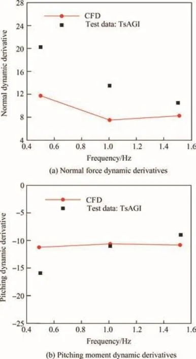
Fig.1 Numerical results of dynamic derivatives compared with experiment data11.

As the reduced frequency continues to decrease,the signs of dynamic derivatives by numerical values are changed in the case,as shown in Fig.2.There are two different interpretations in response to this phenomenon.Sun et al.8found this problem when calculating the Finner model atMa=1.58 in 2011,and explained that when the reduced frequency was lower than 0.008 or greater than 0.150,the errors of numerical simulation increased rapidly,and the identification precision of dynamic derivatives would be relatively poor or even the signs of dynamic derivatives were changed.Wu et al.10also supported this view,and pointed out that when the reduced frequency was very low,unsteady hysteresis effect could not be accurately reflected,which led to an increase of errors.Chen et al.9also found this phenomenon in 2014 when calculating the Finner model atMa=2.1 with the harmonic balance method.He believed that this is a physical phenomenon because when the reduced frequency decreases to a certain extent,the aircraft would change from a dynamic stable state to an unstable state.He pointed out that for a missile with the same shape,its dynamic stability characteristics would change with variations of materials and mass distributions.Yuan et al.4stated his view in the latest paper in 2016:At low frequencies,the dynamic derivatives change rapidly with the oscillation frequency decreases.If the aircraft’s inherent oscillation frequency is low and the calculation of the selected frequency is higher,the prediction would depart from the real situation.

In order to verify which one of the two views is right,the inducement mechanism of these abnormal changes should be studied in depth.Whether a rapid change of dynamic derivatives is numerical or physical,it has lost the referential meanings.Therefore,it is necessary to set a reasonable range span of the reduced frequency.However,there are still no accepted standards for the choice of the reduced frequency in calculating the dynamic derivatives.12

3.Computational methods

3.1.Dynamic derivative equations and computational methods

Taking the calculation of pitching dynamic derivatives as an example,we assume that an aircraft is forced to do a singledegree-of-freedom small-amplitude motion around the center of mass.The given form of the forced oscillation is as follows13:

where α is the instantaneous angle of attack,θ is the pitch angle,α0is the initial angle,αmis the oscillation amplitude,andkis the dimensionless reduced frequency.If the masscenter velocity is constant,the independent variables of the motions in the body axis are the angle of attack α,the pitching angular velocityq,and their respective time derivatives for the longitudinal motions of the aircraft.The pitching moment coefficientCmcan be written as

We assume that the basic flight state is steady,symmetric,and straight with a very modest disturbance amplitude,and only the first-order dynamic derivatives are considered in the calculation.When the aerodynamic forces reach a periodic solution,Cmcan be expressed by Taylor expansion as

Computing the derivation of Eq.(1)yields

Substituting Eq.(4)into Eq.(3),we can get

whereCmθ0is the static stability derivative,whileCm˙θ0is the pitch-damping coefficient.When the reduced frequency is low,Eq.(5)can be approximated as

After the flow field achieves to periodic solutions,the problem of solving the pitch-damping coefficient can be transformed into the problem of how to identifyCm˙θ0from Eq.(5)numerically.Then the following methods can be used.

3.1.1.Integral method

We multiply the operator coskton both sides of Eq.(5),and then by integrating Eq.(5),we can obtain the following formula:

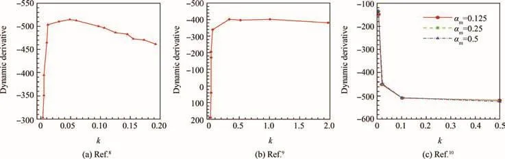
Fig.2 influence of reduced frequency on dynamic derivative.

wheretsis an arbitrary moment after the flow field achieving to a periodic solution,andTis the forced oscillation cycle,

3.1.2.Phase method

Substituting the phases of values 0 and π into Eq.(5),we can obtain

The integral and phase methods are equivalent in mathematics,but the latter is simpler and easier to calculate.However,in numerical computations,the phase method may produce large numerical errors due to the similar number subtraction and the minimum value division in Eq.(8)when the reduced frequency is low.Besides,the identification errors of the phase method are also large since only two points of time-domain data are used in this method.Therefore,the phase method is not commonly used in actual calculations.

3.2.Computational methods of unsteady aerodynamic force

In this study,the aerodynamic forces of an oscillation airfoil are calculated by the Grossmann quasi-steady aerodynamic model and the Theodorsen unsteady aerodynamic model which are based on the potential flow theory,as well as the CFD-based backward difference method in the time domain and the time spectral method.These four computational methods will be introduced in this section.

3.2.1.Analytical potential flow theory models

The results of potential flow theory models can approximate to real results with assumptions of low velocity,incompressible flow,and thin airfoil as well as small perturbation.Then dynamic derivatives can be estimated by the Grossmann quasi-steady aerodynamic model and the Theodorsen unsteady model based on the potential flow analytical theory.

In the Grossmann quasi-steady model,the influence of wake vortices on the airfoil is negligible,and some of the time-memory effects in the unsteady aerodynamic model are also neglected.This model assumes that the aerodynamic forces at any moment only correspond to the state of motion of the airfoil at that moment.Therefore,dynamic derivatives calculated by the quasi-steady model are independent of the reduced frequency,and only depend on the position of the mass center.The expression of the dynamic derivatives is

wherehis the dimensionless distance from the leading edge to the center of mass.

The Theodorsen unsteady aerodynamic model considers the effect of the free vortices of the trailing edge wake and introduces the Theodorsen functionC（k）=F（k）+iG（k）with theassumption thattheairfoiloscillatesharmonically.Dynamic derivatives calculated by the unsteady model are related to the reduced frequency,and the expressions of the dynamic derivatives are14

whereF（k）andG（k）are both functions of the reduced frequencyk,and one can look through the table in Ref.15to obtain the corresponding function values.

3.2.2.Numerical methods

In this paper,the dynamic derivatives of an NACA0012 airfoil are calculated by CFD,and the variation of the dynamic derivatives with the reduced frequency is studied.A program developed by our own research group and called NWIND is used.The computational mesh is a hybrid mesh,and the flow field is solved by thefinite volume method.The central scheme is applied to perform spatial discretization,and the dual time step method is applied to perform time integration.The reliability of the NWIND program has been proven by a number of examples.16,17

Two types of time discretization methods are used for CFD numerical computations.One is the traditional time difference method,and the other is the time spectral method.

The traditional CFD time difference method uses the Backward Difference Format(BDF)for discretization of the physical time step.18The second-order time-accurate BDF is applied in this paper.The time discretization is as follows:

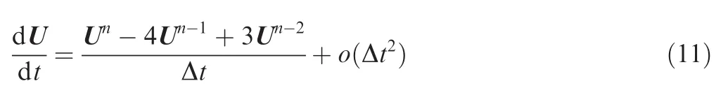
where U is the conservative variables of the flow field,and Δtrepresents the discrete time step.

Since the periodic forced pitching of the airfoil is required to calculate the dynamic derivatives,the flow field has a periodic characteristic.The traditional BDF does not take advantage of this characteristic.The Time Spectral(TS)method assumes that the time history of a flow field is composed of a series of harmonics with different frequencies.Then the periodic unsteady problem is transformed into the coupling ofNsteady-state problems,which greatly improves the computational efficiency.19–21Moreover,the time spectral method has more obvious advantages when the reduced frequency is low.The time discretization of the TS method is as follows19:

whereNis the number of sampling points in a cycle.IfNis odd,then

3.3.Mathematical explanation of abnormal changes of dynamic derivatives

In order to further explain the abnormal changes of dynamic derivativesatlow reduced frequencies,therelationship between the dynamic derivatives and the area of the pitching moment coefficient loop is deduced mathematically.The detailed processes are shown as follows:

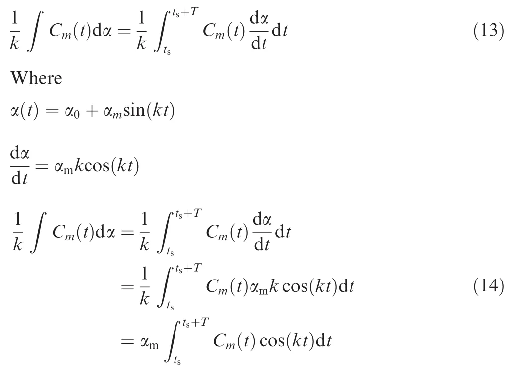
Then,substituting Eq.(7)into Eq.(14),we can obtain

It can be seen from Eq.(15)that the area of the pitching moment coefficient loop is proportional to the reduced frequency,the dynamic derivatives,and the square of the amplitude.As can be seen from Fig.3,when the reduced frequency approaches to zero while the others are unchanged,the area of the pitching moment coefficient loop also approaches to zero.At this point,the solution of dynamic derivatives becomes a problem of the minimum value divided by the minimum value,which would cause a numerical singular phenomenon naturally in the numerical computation.

The pitching motion prescribed about the quarter chord of the airfoil is as follows:

Fig.3 Pitching moment coefficient loops at different reduced frequencies.

where ω is the oscillation frequency.The relationship between the oscillation frequency ω and the dimensionless reduced frequencykis

wherecis the mean aerodynamic chord,andU∞is the freestream speed.The initial flow conditions are shown in Table 1.

4.Test cases and analysis

The NACA0012 airfoil is taken as an example in this paper to conduct numerical simulation,and then the variation of the dynamic derivatives with reduced frequencies,especially low reduced frequencies,is studied.The computational mesh is shown in Fig.4.The total number of mesh cells is 8568;the total number of nodes is 6004;the number of nodes on the airfoil surface is 180;the total height of the boundary layer is 0.02.A standard test case of AGARD2 is used to verify the program,and the calculated dynamic derivatives are compared with the results in Ref.22.

Both the BDF and the TS method are applied to perform time discretization respectively.When the former is applied,each time period is divided into 120 time steps,and a total of 4 cycles are computed.When the latter is applied,seven time points are selected in one cycle.The pitching moment coef ficient loops of the computed lift and moment coefficients are compared with experimental and literature values,as shown in Fig.5.Table 2 lists the dynamic derivatives calculated by the integral method in this paper along with the results in Ref.22.It can be seen that the results computed by our program are coincident well with the literature results and the experimental data.Therefore,the calculation results of this program are reliable.

In order to study the problem of numerical errors in computing dynamic derivatives at low reduced frequencies,the variation of the dynamic derivatives of the NACA0012 airfoil at low-velocity and incompressible cases as well as small perturbation with reduced frequencies is calculated by CFD,and then numerical results are compared with those of the Grossmann model and the Theodorsen model.The initial conditions areMa=0.2，α0=0°，αm=2°，Re=4.8 × 106.The position of the rigid axis is set at the quarter-chord.The influences of different methods and different convergence accuracies on the calculation results are studied.

4.1.influences of different numerical methods on computational results

The BDF and the TS method are applied to time discretization in the CFD solution.Each time period is divided into 120 time steps,and a total of 4 cycles are computed in the time domain difference method.Seven time points are selected in one cycle in the TS method.The integral method and the phase method are applied to extract dynamic derivatives.On the whole,there are four numerical methods to solve dynamic derivatives,as shown in Table 3.

The convergence criterion is 5.0×10-8.The variations of the dynamic derivative with a reduced frequency by different solutions are shown in Fig.6.As can be seen from the figure,the dynamic derivatives of both Algorithms 1-1 and 1-2 appear exponential divergence when the reduced frequency is lower than 10-3,and then numerical errors have resulted innonphysicalresults.In Algorithm 2-1,an exponential divergence of the dynamic derivative appears when the reduced frequency is lower than 10-4.Only Algorithm 2-2 does not show a numerical divergence.However,as the reduced frequency continues to decrease in Fig.7,the dynamic derivative of Algorithm 2-2 also shows an exponential divergence when the reduced frequency is lower than 10-5.Therefore,as the reduced frequency decreases,a numerical divergence is inevitable.However,it can be mitigated by combining the TS method with the integral method.

Table 1 Initial flow conditions of the standard test case.

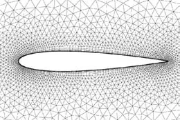
Fig.4 Near- field mesh for the NACA0012 airfoil.

Fig.5 Comparisons of the lift and pitching moment coefficient loops with the data of Ref.22.

Table 2 Comparisons of dynamic derivatives of AGARD2 with reference data.

Table 3 Four numericalmethods to solve dynamic derivatives.

Fig.6 Variations of dynamic derivative with a reduced frequency using different algorithms.

For the BDF,the truncation error of the time discretizationo（Δt2）will increase and the precision will decrease when the reduced frequency decreases in the condition that the number of time steps is constant in one period.However,for the TS method,the above situation does not happen because the truncation error of the time discretization is in the frequency domain.For the integral method and the phase method,both will show obvious rounding errors due to the minimum value divided by the minimum value when the reduced frequency is very low,but for the phase method,numerical errors would be relatively larger.Therefore,in the latter test cases,without any special instructions,we use the TS method and the integral method in order to make the algorithm more reliable at low reduced frequencies.

Fig.7 Numerical divergence of algorithm 2-2.

Fig.8 influence of convergence accuracy on computation of dynamic derivative.

4.2.influence of convergence accuracy on computational results

We analyze the numerical divergence of dynamic derivatives as decreasing the reduce frequency at different convergence accuracies of 5.0×10-6,5.0×10-7,and 5.0×10-8.Computation results are shown in Fig.8.As can be seen from the figures,a numerical abnormal fluctuation appears when the reduced frequency is lower than 10-3in the case that the convergence accuracy of CFD is 5.0×10-6.The numerical fluctuation is mitigated until the reduced frequency is lower than 10-5in the case with a convergence accuracy of 5.0×10-7.Furthermore,when theconvergenceaccuracy isincreased to 5.0×10-8,a numerical divergence still appears as the reduced frequency is lower than 10-5.The results demonstrate that there are two kinds of numerical error result in numerical fluctuation or divergence.One is the convergence accuracy and truncation errors of CFD in computing aerodynamic loads,and the other is the round-off error amplified due to the minimum value divided by the minimum value when obtaining dynamic derivatives.With a convergence accuracy from 5.0×10-7to 5.0×10-8，the numerical divergence is not mitigated because the numerical errors are mainly from the latter.

4.3.Law of dynamic derivative variation with reduced frequency at different Mach numbers

In order to determine the appropriate range span of the reduced frequency in calculating the dynamic derivative,the variations of the dynamic derivative with the reduced frequency at different Mach numbers are studied in this paper.Three different Mach numbers,Ma=0.2，Ma=0.8 andMa=1.8,are chosen to simulate subsonic,transonic,and supersonic conditions,respectively.The rest of the flow conditions are the same as in Section 4.1.Results are shown in Figs.9 and 10.It can be seen from Fig.10 that when the reduced frequency is lower than 10-4,the dynamic derivatives change rapidly as the reduced frequency decreases in the conditions of transonic and supersonic cases.Therefore,in the calculation,the reduced frequency should not be too low.Furthermore,we can also see from Fig.10 that,for the subsoniccase,thedynamicderivativemaintainsnearly unchanged when the range span of the reduced frequency is 10-2–10-4,while for the supersonic case,the range span is 10-1–10-3.However,for the transonic case,the dynamic derivative variation with the reduced frequency is more obvious.The change of the dynamic derivative is relatively moderate when the range span of the reduced frequency is 10-2–10-3.

To sum up,when the range span of the reduced frequency is 10-2–10-3, the dynamic derivative maintains nearly unchanged,and the numerical errors are small.The dynamic derivatives have a referential meaning.

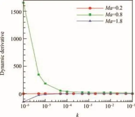
Fig.9 Change law of dynamic derivative with reduced frequency at different Mach numbers.

Fig.10 Detailed figures about change law of dynamic derivative with reduced frequency at different Mach numbers.

5.Conclusions

(1)The area of the pitching moment coefficient loop is proportional to the reduced frequency,the dynamic derivative,and the square of the amplitude.As the reduced frequency approaches to zero,the area of the pitching moment coefficient loop also approaches to zero.The situation that the minimum value divided by the minimum value results in numerical singularity when calculating dynamic derivatives at very low reduced frequencies.

(2)Comparing numerical values with analytical values,wefind that the divergence of the dynamic derivatives at low reduced frequencies is caused by the numerical singularity.By using the time spectral method and the integral method,the numerical divergence of the dynamic derivatives at low reduced frequencies can be effectively mitigated,but cannot be avoided.

(3)There are two sources of numerical errors in computing the dynamic derivatives at low reduced frequencies:the numerical errors of CFD in the computation of aerodynamic loads and the numerical errors of the method to obtain the dynamic derivatives.The numerical divergence of the dynamic derivatives at low reduced frequencies cannot be avoided just by increasing the convergence accuracy of CFD.

(4)By numerical computation and study on the variations of the dynamic derivative with the reduced frequency at different Mach numbers,wefind that when the range span of the reduced frequency is 0.001–0.01,the dynamic derivatives at different Much numbers maintain nearly unchanged,which have a referential meaning.

Acknowledgements

This study was co-supported by the National Science Foundation forDistinguished YoungScholarsofChina(No.11622220)and the Programme of Introducing Talents of Discipline to Universities(No.B17037).