The effects of mean sea level rise and strengthened winds on extreme sea levels in the Baltic Sea

Magnus Hieronymus*, Christian Dieterich, Helén Andersson, Robinson Hordoir

Swedish Meteorological and Hydrological Institute, Folkborgsvägen 18, Norrköping, Sweden

Keywords:Extreme sea levels Sea level rise Wind speeds Baltic Sea

A B S T R A C T Mean sea level rise and climatological wind speed changes occur as part of the ongoing climate change and future projections of both variables are still highly uncertain. Here the Baltic Sea's response in extreme sea levels to perturbations in mean sea level and wind speeds is investigated in a series of simulations with a newly developed storm surge model based on the nucleus for European modeling of the ocean (NEMO)-Nordic. A simple linear model with only two tunable parameters is found to capture the changes in the return levels extremely well. The response to mean sea level rise is linear and nearly spatially uniform, meaning that a mean sea level rise of 1 m increases the return levels by a equal amount everywhere. The response to wind speed perturbations is more complicated and return levels are found to increase more where they are already high. This behaviour is alarming as it suggests that already flooding prone regions like the Gulf of Finland will be disproportionally adversely affected in a future windier climate.

Extreme sea levels and how those are affected by climate change is a major issue for coastal communities around the globe. Our focus here is on the Baltic Sea, a semi-enclosed and brackish basin that is connected to the North Sea via the narrow Danish Straits. Large parts of the Baltic sea coast is densely populated and its drainage area is home to 85 million inhabitants[1]. Moreover, several major cities are situated on the Baltic Sea coast including the capitals of Denmark, Sweden, Finland, Estonia and Latvia. Large property values as well as invaluable historical buildings are therefore increasingly at risk from flooding as the sea rises.

Tides and North Atlantic storm surges are quite efficiently filtered by the Danish Straits and the sea level variability in the Baltic Sea is consequently primarily wind driven [2]. Much of the earlier work on sea level variability in the Baltic Sea has focused on quantifying and understanding its driving forces and accociated time scales [3-6]. Our focus here is on extreme sea levels and how those are affected by climate change. Some earlier work on that topic includes a study by Meier et al. [7] who looked at changes in the 99% quantiles of sea level and a study by Gräwe and Burchard [8] who looked at the changes in return levels in the Western Baltic Sea, both using a combination of different climate scenarios and sensitivity experiments. Most earlier work on the response in extreme sea levels to climate change have focused primarily on analysing dynamical downscalings of climate simulations ran with different emission scenarios. Our aim here is to take a more direct approach. Instead of perturbing key climate parameters like the greenhouse gas forcing we will directly perturb key parameters for sea level extremes. The most prominent such parameters for the Baltic are wind speeds and mean sea level rise [2]. This more direct approach is a good complement to the aforementioned, since it allows us to quantify the sensitivity of sea level extremes to its key drivers. This is normally not possible when using climate scenarios because of the inherent complexity in the response of, for example, wind speeds to increases in greenhouse gas forcing. Our aim here is thus not to predict the return levels in a possible future climate,but rather it is to understand how the return levels change as a function of their forcing. Such sensitivity experiments have proven invaluable for understanding a vast range of physical phenomenon such as the meridional overturning circulation,the oceanic heat transport and double diffusive convection to name but a few (see Refs. [9-11]). However, sensitivity experiments on extreme sea levels are in short supply and as a consequence so is our understanding of the physics that govern them.

The most ambitious sensitivity experiments yet undertaken for return levels in the area are those for the Western Baltic Sea by Gräwe and Burchard [8], where they probed the effects of raising the mean sea level by either 0.4 or 0.8 m and in a separate run increasing the wind speeds by 5%. Together with a control run this makes a total of four experiments. We have conducted a total of 16 sensitivity experiments where the mean sea level is increased between zero and one meter and the wind speeds between zero and 15%. These 16 experiments are then used to calibrate a simple linear model with only two tunable parameters that accurately estimates the effects of wind speed increases and mean sea level rise on return levels throughout the Baltic Sea.

Our experiments are done using a barotropic version of the nucleus for European modeling of the ocean (NEMO)-Nordic model [12]. This type of model is, due to its cheap computational cost, often used for sea level modelling [13-15]. Our model setup is identical to that used in Ref. [2], where more info on the model performance and parameter choices are given. The horizontal resolution is two nautical miles and the model grid covers the Baltic Sea and parts of the North Sea. The model is forced with a dynamically downscaled ERA40 forcing [16]. The downscaling is done using RCA4 [17, 18] to a resolution of 11 km for the years 1961 to 2005. River run-off data comes from the hYdrological predictions for the environment (HYPE) model [19]. The open boundary condition consists of 9 tidal harmonics and wind-driven sea level from a simple coarse resolution barotropic storm surge model covering a large part of the North East Atlantic. Instantaneous sea level data is stored every hour.

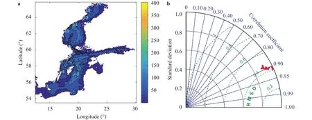
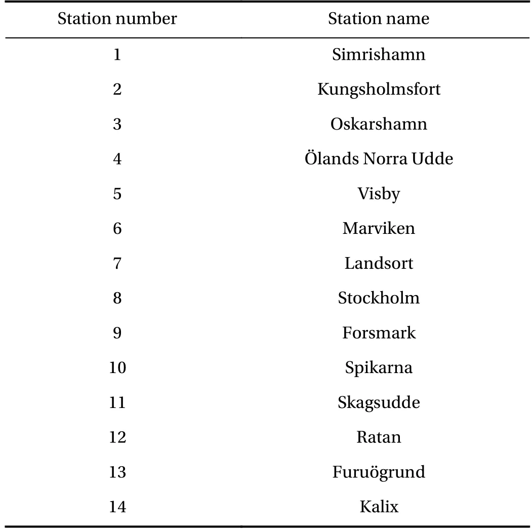
Swedish Meteorological and Hydrological Institute (SMHI)operates several long term sea level observation stations along the Swedish Baltic Sea coast where hourly sea level observations are made. To evaluate the model's performance against observations we have chosen the period between the years 1996 and 2005 during which we have continuous hourly data from 14 different stations. The location of these stations as well as a map of the model bathymetry are shown in Fig. 1(a), and the station names are given in Table 1. The right panel shows a nondimensional Taylor diagram comparing observed and modelled sea levels at the 14 stations. All stations are highly correlated with the observations, and the standard deviation of the modelled sea level is generally around 90% of the observed one. The Taylor diagram gives a good integrated view of the model performance but are not particularly informative on the performance for extreme sea levels.

Fig. 1. Bathymetry with depths in meters and the location of the sea level measurements stations (a) and nondimensional Taylor diagram of the sea level performance at the stations (b). The names of the stations numbered 1-14 are found in Table 1. The nondimensionalization of the model's rms error and standard deviation is achieved through division by the observed standard deviation at the respective station.

Table 1 The names of the measurements stations shown with numbers in Fig. 1.

To evaluate the performance for extremes we have calculated 10, 20, 30, 40, and 50 year return levels from the model and the observations. To get accurate return level estimates one needs long datasets and we have therefore chosen to do this comparison at the seven observation stations that have data coverage for the full 1961-2005 period. Return levels are estimated using the annual maxima method1Here we use a climatic year (a year that begins July 1 and ends June 30).[8, 20], where a generalized extreme value distribution [21] is fitted to the time series of annual maxima. The return levels are then calculated from the inverse cumulative distribution function using software from Matlab's statistics toolbox. Table 2 shows the 10 and 50 year return levels derived from the model run and the observations. The average model error, assuming the observationally based estimate is flawless, in the 10 year return level is less than 4 cm, while that in the 50 year return level is less than 7 cm. The 20, 30, and 40 year return levels have model errors that are intermediate between these two. The model produces nearly as many over- as underestimates of the return levels and there is a good overlap of the confidence bounds at all stations. In fact, the model estimates of the return levels are within the confidence bounds of their observationally based counterparts for all return levels and stations with the exception the 50 year return level at Stockholm,where the model estimate is 2 cm below the confidence bound of the observational estimate.

A total of 16 simulations are performed, with four different initial area averaged sea levels, and four different factors multiplying the wind speeds in the forcing fields. Our experiments thus perturb the wind speed, but not its direction. For extreme sea levels this means that we model the conditions that would occur if storms were stronger than they are in today's climate,but still occur with similar frequencies and spatial distributions as they do today. The simplicity of these perturbations is essentially what differs our forcing from a climate scenario, and this difference is absolutely key for understanding the relationship between extreme sea level and their forcing.

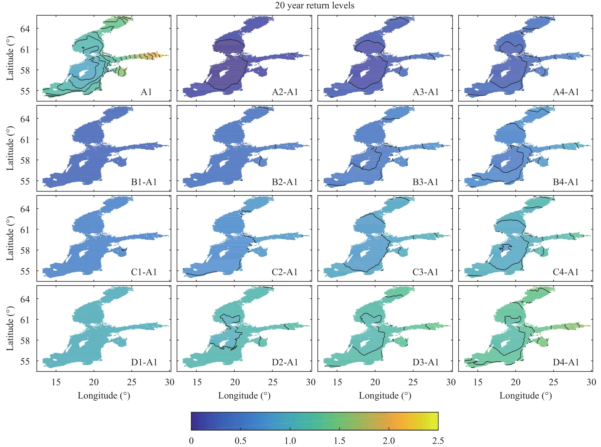
The nomenclature used for our simulations is as follows: A,B, C, and D are used for the initial sea level perturbations and correspond to a sea level rise of 0, 0.33, 0.66, and 1 m. The wind speed perturbations are dubbed 1, 2, 3 and 4 and correspond to the multiplication of the wind field by a factor,, equal to 1,1.05, 1.10 or 1.15. Our simulation called A1 is thus the unperturbed version, while the run called D4 is initiated with 1 m of extra water and have wind speeds increased by 15%.

Figure 2 shows the difference in the 20 year return levels in our different experiments. We can see from the A1 panel that there is a general pattern of smaller return levels over much of the Swedish east coast, and larger ones in the bay of Bothnia, the gulf of Finland and the gulf of Riga. This general pattern is in good agreement with Ref. [7], and the spatial pattern is consistent also for the 10, 30, 40 and 50 year return levels. It is also consistent with what we know about the sea level dynamics in the Baltic since these areas of high return values correspond to known antinodes of Baltic Sea seiches [3, 22].

The first column of Fig. 2 shows the return level changes induced by just a mean sea level change, and it is clear that the response is very nearly linear with a spatially constant coefficient of proportionality equal to one. That is, increasing the mean sea level by 1 m gives a very similar increase in the return level everywhere. The Study by Gräwe and Burchard [8] also found a linear response to mean sea level changes, but with spatial differences in their coefficient of proportionality of up to 10% in their study in the Western Baltic. Our more uniform response is likely a consequence of the courser resolution in our model, deviations from unity in the coefficient of proportionality are therefore expected only in shallow or narrow areas beyond the reach of our current configuration.

The response to wind speed perturbations is also nearly linear, however, here we find large spatial differences in the coefficient of proportionality. Linear regressions of the return level separately on the windspeed and mean sea level perturbations in each gridbox gives a coefficients of determination,that is very close to one everywherefor wind speed perturbations andfor mean sea level perturbations) so a large majority of the variance is explained by these linear mod-els. The linearity of the response can be used to approximate the return level at any given location in the Baltic Sea as a function of wind speed and mean sea level perturbations according to

Table 2 10 and 50 year return levels from observation and the model. Values in square brackets are likelihood-based 95% confidence intervals.The subscript on RL indicates which return level it is and the superscript whether the value is calculated from the model or the observations.

Fig. 2. Difference in 20 year return levels from our different experiments. The label A1 indicates that it is the return level from the unperturbed run, and A2-A1 indicates that we see the return level from the A1 subtracted from that in A2 and so forth. Contours are drawn every 0.1 m.

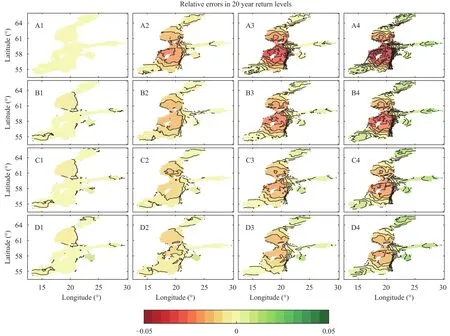
The relative errors in the 20 year return levels, defined as the difference between the return level calculated from the model data and that given by Eq. (2) divided that calculated from the model data, is shown in Fig. 3. There is a tendency of the linear model to underestimate high- and overestimate low return levels, albeit with very modest relative errors typically smaller than 1%. The largest errors are found in the A4 panel where the average of the modulus of the relative error equals 1.6% and the average of the modulus of the error is 3 cm. The error distribution is dependent on the cost function and our choice to minimize the sum of absolute errors is one of many possible choices. One can, for example, easily create a linear model that performs better in specific locations by creating a cost function that penalizes errors more strongly at those. An obvious such option is to improve coastal return levels on the expense of open sea values. However, the errors of the current linear model are already small enough that the estimated return levels are typically well within the confidence bounds of those derived from the model and we have hence not pursued using alternative cost functions.

Fig. 3. Relative errors in 20 year return levels given by the linear model. Contour intervals are 0.005.

The Baltic Sea's response in extreme sea levels to perturbations in mean sea level and wind speeds were examined in a large suite of sensitivity experiments. Our main finding is the simple and accurate parametrization of the return levels. The strength of this expression lies in its universality and simplicity.The universality stems from the fact that the spatially dependentcan be accurately parametrized as a linear function of.Plainly speaking this means that return levels increase more with increasing wind speeds at locations where they are already large.This alarming behaviour is particularly problematic in the Gulf of Finland where high return levels are found in the vicinity of the major cities Saint Petersburg and Helsinki. Moreover, it may affect the life time of the Saint Petersburg Dam [23] as an effective flood protection if our future climate turn out to be windier than our present.

The near linearity in the response to mean sea level rise is likely quite universal, in the sense that we would expect a similar response in many other ocean environments. Whether the nearly linear response to wind speed perturbations is universal is more questionable. The wind stress that goes into the momentum equations typically depends on the wind speed squared or even cubed [24-26], so departures from linearity will certainly be seen for large enough perturbations. The most interesting question of universality is whether the key result for the Baltic Sea, that the spatial dependencecan be accurately parametrized as a linear function of, holds true also in other areas. The sea level variability in the Baltic Sea is dynamically simple compared to that in many other ocean environments, being mostly wind driven and governed by standing waves [3, 22,27], socould certainly behave differently elsewhere. An obvious and important next step is therefore to see whether this type of parametrisation is applicable also outside of the Baltic Sea in coastal areas around the world.

We believe that our simple parametrisation can prove useful for future coastal planing as a complement to the more traditional approaches based on climate scenarios [28]. Both the wind speeds and the mean sea level are highly uncertainty in climate projections for the 22nd century [29-31]. The parametrisation could therefore be used to create simplistic high or low end return level projections based on the range of wind speed and mean sea level changes seen in the climate projections. The linearity in the response to mean sea level rise is also useful because the Scandinavian Peninsula is still experiencing a significant and spatially varying post glacial rebound. This means that realistic mean sea level rise scenarios will affect different parts of the Baltic Sea coast differently, but post glacial rebound is not included in the current generation of climate models and the linear response makes it easy to correct for that omission posthum-ously.

Acknowledgements

The work has received funding from the project “Future flooding risks at the Swedish Coast: Extreme situations in present and future climat”, Ref. No. P02/12 by Länsförsäkringsbolagens Forskningsfond, and through the Swedish Civil Contingencies Agency (MSB) through the project“Hazard Support: Risk-based decision support for adaptation to future natural hazards”.