计量经济学下下分析新生儿出生体重决定因因素

张 宇

（长江职业学院院 财会金融学院，湖北 武汉 430000））

计量经济学下下分析新生儿出生体重决定因因素

张 宇

（长江职业学院院 财会金融学院，湖北 武汉 430000））

衡量一个新生儿健康成成长的标志有很多，可以是婴儿的身高、体重、头围围、胸围等，其中体重和身高最具有代表性和可比较性。通通常一个新生儿的体重在2.5公斤到4公斤，有的时时候女婴儿的体重甚至会高于男婴。到底影响新生儿体重的的因素有哪些呢，本文将通过对1300余名新生儿体重重、父母受教育程度、母亲孕期抽烟程度、家庭收入等数据据进行多元回归分析，结合 EViews软件得到影响因因素变量模型及程度，最终得到的结论是，婴儿出生体重与与母亲受教育程度成正比，孕期抽烟与体重成反比。。

新生儿体重；决定因素素；计量经济学；多元回归；EViews

The weights of the newborns aree quite different,usually can be heavier or lighter bbetween 2.5 to 4kilogram.Sometimes a girl’s birthweight can be heavierthan a boy, why? In this paper,, wewill explain child birth weight in terms of varioous factors and results from the application ofeconommetric methods.

I. Data description

Data in series bwght containsinformation on 1,388 births, but there are data misssing in fathedu,only 1192 births included in nullhypothesis. In details, bwght is birth weight, ouncces, faminc is annual family income, fatheduc is yeaars of schooling for the farther, the same way,motheedduc is years of schooling for the mother, cigs is aveerage number of cigarettes the mother smoked peer day during pregnancy, lbwght is log of bwght annd lfaminc is log of faminc. And then let’s see the hissttogram and XY scatter plot due to these variables.

Figure 1.1: Histogram off birth weight(新生儿体重的柱柱状图)

According to Figure 1.1,we can see that birth weight distribution is almost syymmetric. Data mean is in the middle, but few birth wweights are more than 200, ounces.

Figure 1.2: Histogram of lbwgg ht(lbwght柱状图)

As shown in Figure 1.22, the distribution of lbwght is asymmetric, data meaan is 4.76 which areon the right side and the tail develoopment is different.

Figure 1.3: “Family income—birth weigght”scatter plot(家庭收入——新生儿体重散散点图)

From Figure 1.3, the data is moore concentrated in family income 0-20. The more inccome the family gets the bigger range of birth weightt. Some outliers can be ignore

Figure: 1.4 “lfaminc — bwght” sccatter plot（lfaminc — bwght散点图图）

As shown in Figure 1.4, the moree the lfaminc is,the lower the bwght is. The trendisdecreasing to some extent. And the data is more cconcentrated on lfaminc 2 to 4.

Figure 1.5: “Father education — birth weeight” scatter plot（父亲受教育年数——新生儿体重重散点图）

According to Figure 1.5,thetrend of birth weight is increasing as years of faather education increasing. And the range of birthweight is also increasing.

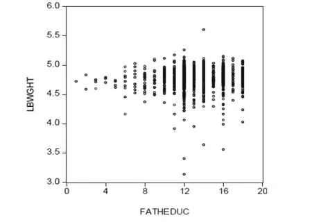
Figure 1.6: “Father Education——lbwght” scatter plot(父亲受教育年数——lbbwwght散点图)

From above Figure 1.6, tthere is also a small increasing trend in lbwght and tthe same in therange.

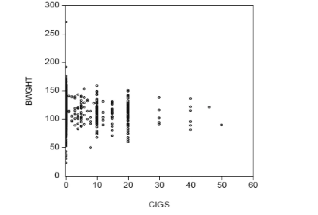
Figure 1.7: “Cigs — birth weeight” scatter plot（母亲孕期吸烟数量——新生生儿体重散点图）

As shown in Figure 1.7, thhe trend is decreasing,the more cigarettes the mothher smoked per day during pregnancy, the lighter thhe birth weight will be and the same as the quantityy. The data is more concentrated when cigs is smalll than 10.

Figure 1.8: “Cigs—lbwght” scattter plot（母亲孕期吸烟数量——lbwght散点图）

According to Figure 1.7 and 1.8,, we can see that the situation is almost the same.

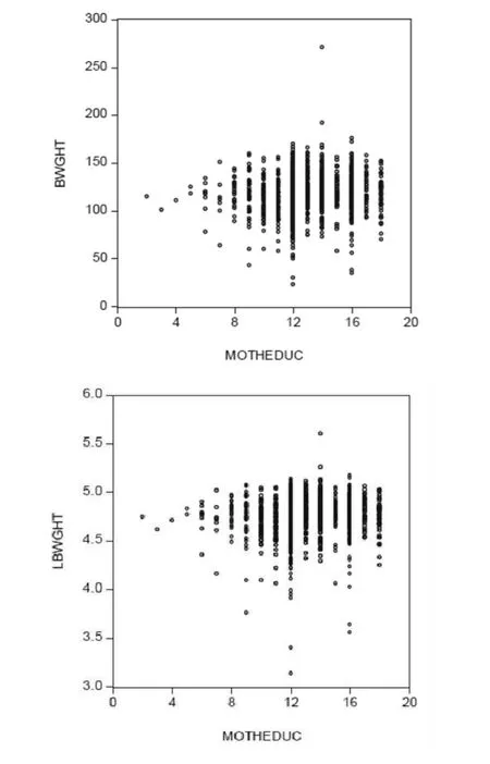
Figure 1.9: “motheduc—bwghht” and“motheduc—lbwght” scatterr plot（母亲受教育年数与bwght、lbwghht散点图）

From Figure 1.9, the range of bbwght is bigger,and more concentrate on mothedcuu from 8 to 18 years. And nearly the samesituation in“lbwght-motheduc” scatter plot.

Ⅱ. Economic relationshipp

In this section, we will dettermine the dependent and independent variables acccording to covariance analysis and to see if there iis a multicollinearity problem in the variables or not.

Table 2.1: Correlation matrixx（相关系数矩阵）

From table 2.1 correlation mmatrix, correlation between independent variabless and bwght is higher than correlation between indeppendent variables and

lbwght, which is corr(x,bbwght) is higher thancorr(x,lbwght). So wee can determine that

dependent variableis bwght.

And then we can find inthe red part of Table 3.1, between independent vaariables faminc and lfaminc, corr(lfaminc,bwghht)which equals to 0.818 is higher than corr(famminc,bwght)which is 0.80. So we can remove famincand keep lfaminc.

HO:corr(x1,x2)=0H1:ccorr(x1,x2)≠0

And p-values of lfamminc, fatheduc and motheduc are all small thanor around 10%, but correlation between lfaminc, faatheduc and bwght are higher than 70%, thereis multicollinearity problems，weremove lfaminc aand fatheduc.

So we’ve got independentvariables bwght,dependent variables motheducannd cigs.

The more cigs mother smmoked per day during pregnant can lead to the decrrease of birth weight because of the loss of health II think. And the more family income is, the healthier oof the mother may be,which may give birth to a heaviier child.

Ⅲ. Methodologyand estimmation

According to the correlattion analysis, we can estimate a theoretical regressioon model with chosen variables as follow:

bwght= βO+β1cigs+ββ2mothereduc+u(3.1)

Variables are described in chaptee r 2.

Since we have the theoretical moodel, we can get estimate model form EViews by oppen variables as equation:

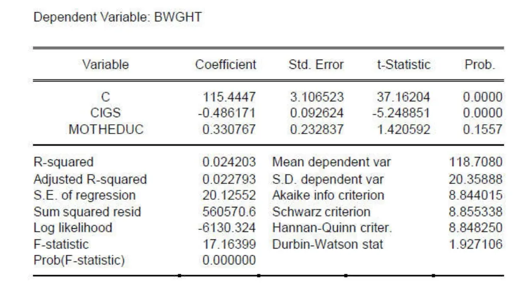
Table 3.1: Least squares (最小二二乘法)

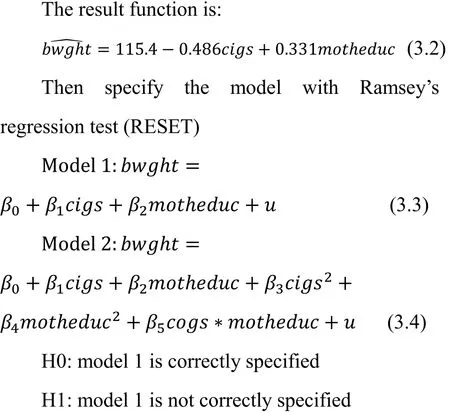
Table 3.2: Ramsey’s RESET test iin EViews（拉姆齐回归设定误差检验验）

From Table 3.2, we’ve got the pprobability 7.2%which is smaller than 10%, reject HH0 which means model 1 is not correctly specified. TThen we need to include quadratic forms of independennt variables.

Table3.3: New Leastt Squares（新的最小二乘法法分析）

Table 3.4: New Ramsey’’s RESET test（新拉姆齐回归设定误误差检验）

As shown in the Table 33.4, the probability is only 1.7%. Compared the situaation in Table 3.2, it seems that model 1 is more sppecified, we will use model 1.

Ⅳ. Econometric verificcationand Statistical inference

After estimation, incase we have heteroscedastic error term,we will test the heteroscedasticity of thee model. White heteroscedasticity test can be ussed.

H0: errors are homoscedasstic

H1: errors are heteroscedasstic

Table 4.1:White heteroscedasticitty test（异方差检测）

In the Table 4.1, p-value iss 36% which is higher than∝, 10%. So we fail toreject H0.Errors are homoscedastic, there isn’tt heteroscedasticity problem.

And then, we will conduct hyppothesis testing regarding the significance of essttimated model parameters.

Two-side hypothesis testingin a multiple regression model,

115.4 -0.486cigs+0.331motheduuc (4.1)

Degrees of freedom = n - k - 1== 1388– 2 – 1=1385, from Excel we can get tcequaals to 1.646 by function T.INV.2T (0.1, 1385).

Table 4.2: Coefficient of determinationn in a multiple regression model in EViewws(多元回归模型中的决定系数数)

Figure 4.1 Two-sided hypothesis testing off β1(β1 双边检测)

In Figure 4.1, we can see that t-sstatistic for β1 is in the tail, so we reject null hypothhesis. And that means x1, cigs, is statistically significcant at the 10%level.

Figure 4.2 Two-sided hypothesis testing off β2(β2 双边检测)

From Figure 4.2, t-statistic forβ2is not in the tail, so we reject null hypothesis. Annd which seems that x2, motheduc, is not so statisticallly significant at the 10% level. The difference is noot very far from 1.646, so we can accept H0.

Next, we will conduct the signn ificance test of overall model.

R2is called the coefficieent of determination,shows how much changes in thhe dependent variables can be explained by using inndependent variables.The significance of R2is testedusing F-statistic.

Table 4.3: Goodness of fit test in EVViews（拟合优度检验）

As we can see in Table 88.1, the probability of F-statistic is 0, smaller than 110%. F-statistics is in the tail, we have to reject H00. So we conduct the determination of bwght model iss overall significant.

Ⅴ. Economic verificationn and Interpretation

Now we have got the finalmodel:

115.4 -0.486cigs+0.331mootheduc(5.1)

In details, one unit inccreasing in average number of cigarettes the motther smoked per day during pregnancy, 0.486 unnit decrease of the newborn’s birth weight; onne unit increase of motheduc will lead to 0.3331 units increase in dependent variable birth weightt.

If average number of ccigarettes the mother smoked per day during preggnancy is increasing,infant health will be influenceed and get a smaller birth weight; Inversely if the mmother education years are longer, she may have a bettter gene and be more patient to her baby. R2showws 2.4% our model explains in birth weight usingg the information on dependent variables.

Ⅵ. Conclusion

Review the whole projecct, a newborn’s birth weight is determined by the nuumber of cigs mother smoked during pregnancy, thhe education year of mother.

If you want a heavier cchild to some extent,you’d better have a better education and don’t forget to smoke less during pregnant.

Bibliography（参考文献）

[1]. JeffreyM.Wooldridge. Introductory econometrics: A modern approach:现代观点[M]. 清华大学出版社, 2004.

[2]. Stock J H, Watson M W. Introduction to econometrics. [J]. American Statistician, 2003,45(6):págs. 223-226.

[3]. Newcombe R G. Cigarette smoking in pregnancy.[J]. British Medical Journal, 1976,2(6038):492-492.

[4]. Econometric lectures at VSB-Technical University of Ostrava

On Determinants of Birth Weight for Newborns under Econometrics

Zhang Yu
（Changjiang Polytechnic College Wuhan 430000 Hubei）

There are a lot of signs of measuring the growth and development of newborns,such as height,weight, head circumference, chest circumference, etc., of which the weight and height are the most representative. Generally, the weight of a newborn is about 2.5kilos to 4kilos,and sometimes, the weight of the girl is heavier than that of a boy. What are the elements to affect the weight of newborns? The paper would make a multiple regression analysis on the following data such as their weight, parents’ education, the smoking degree of the pregnant mother and family income, etc. in more than 1300 newborns. Connecting with EViews software, we have got the variablemode and degrees of affecting factors. The final conclusion is that the birth weight of newborns is inversely proportional tothe mother’s education, and the smoking pregnant period is inversely proportional to their birth weight.

Weights of newborns; Determinants; Econometrics; Multiple regression;EViews

R723.19 文献献标识码：A

1672-1047（2017）005-0108-06

10.3969/j.issn.1672-1047.20117.05.32

* 收搞日期：2017-09-20

张宇，女，湖北红安人，金融学学硕士，教师。研究方向：主要从事经济学研究。

[责任编辑：张克新]