Exact Boundary Observability for a Kind of Second-Order Quasilinear Hyperbolic Systems∗
2016-06-05KeWANG
Ke WANG
1 Introduction
As a dual problem of controllability,the exact boundary observability for linear wave equations has been deeply studied(see[10–12,18]).Based on the theory of semi-global classical solutions to quasilinear hyperbolic systems(see[6,9]),by a constructive method,Li et al.[4,7–8]obtained the exact boundary observability for quasilinear hyperbolic systems.Later,Li[3,5]and Guo and Wang[1]discussed the exact boundary observability for autonomous and nonautonomous 1-D quasilinear wave equations,respectively,and showed the implicit dualities between the corresponding exact boundary controllability and the exact boundary observability.For the general 1-D quasilinear hyperbolic equation utt+a(u,ux,ut)utx+b(u,ux,ut)uxx=c(u,ux,ut),where u is the unknown function of(t,x)and(a2−4b)(0,0,0)>0,Shang and Zhuang[13]established the corresponding local exact boundary observability,including the 1-D quasilinear wave equation as its special case.
For second-order quasilinear hyperbolic systems,there are few results on the exact boundary observability.Yu[16]considered the second-order quasilinear hyperbolic system utt+(A+B)(u,ux,ut)utx+AB(u,ux,ut)uxx=F(u,ux,ut),where u=(u1,···,un)Tis the unknown vector function of(t,x),matrices A and B have only n positive eigenvalues and n negative eigenvalues,respectively.By a constructive method,she obtained the local exact boundary observability.Later,for a quasilinear coupled hyperbolic system
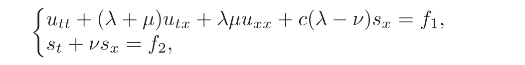
where λ(0)<0,μ(0)<0,ν(0)>0,she got the exact boundary observability by using similar constructive method and applied this result to a first-order quasilinear hyperbolic system of diagonal form and proved that the exact boundary observability is still valid even though the boundary conditions are not coupled(see[17]).
Recently,for a kind of coupled system of 1-D quasilinear wave equations:
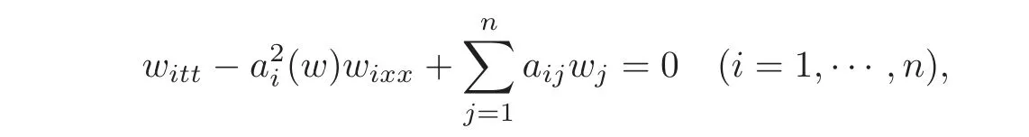
where w=(w1,···,wn)Tand ai(0)>0(i=1,···,n),the authors of[2]discussed the local exact boundary observability with various types of boundary conditions and showed the implicit dualities between the exact boundary controllability and the exact boundary observability.
In this paper,we continue to consider the kind of second-orderquasilinear hyperbolic systems proposed in[14].Based on the known result on the existence and uniqueness of semi-global C2solution to this kind of systems(see[14]),by using a constructive method,we discuss the exact boundary observability and show the implicit dualities between it and the corresponding exact boundary controllability given in[14].The conclusions in both[2]and[13]are of its special cases.
Consider the following kind of second-order quasilinear hyperbolic systems:

where u=(u1,···,un)Tis the unknown vector function of(t,x),A(u,v,w)=(aij(u,v,w))and B(u,v,w)=(bij(u,v,w))(i,j=1,···,n)are both n×n matrices with smooth entries,and have n real eigenvalues and a complete set of left eigenvectors on the domain under consideration,respectively.Suppose furthermore that

Thus,there exists an invertible n×n matrix L(u,v,w)such that
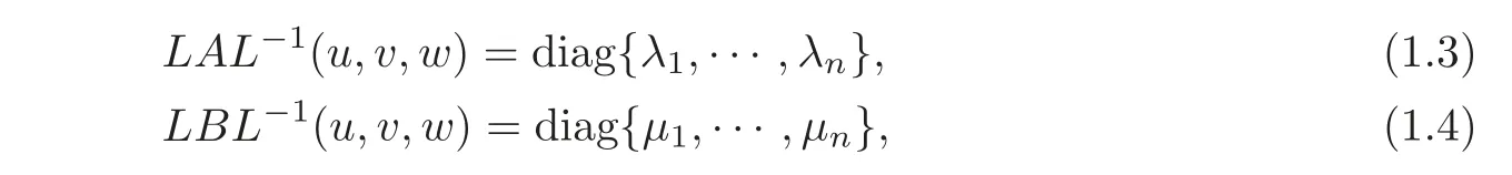
where λ1,···,λnand μ1,···,μnare the real eigenvalues of matrices A and B,respectively,and L=(lij)is just the matrix composed by the common left eigenvectors of A and B.Moreover,we assume that on the domain under consideration

and

In addition,C=C(u,v,w)=(c1(u,v,w),···,cn(u,v,w))Tis a smooth vector function with

By[14],system(1.1)has 2n real eigenvalues

This paper is organized as follows.In Section 2,we recall the existence and uniqueness of semi-global C2solution to the second-order quasilinear hyperbolic system(1.1)under different cases.Then the two-sided and one-sided exact boundary observability are discussed in Section 3,respectively.Finally,in Section 4,we present an implicit duality between the exact boundary controllability and the exact boundary observability.
2 Existence and Uniqueness of Semi-global C2Solution
In this section,we recall brie fly the result on the semi-global C2solution to the second-order quasilinear hyperbolic system(1.1)under different cases in[14].
For system(1.1),we give the following initial condition:

where ϕ =(ϕ1,···,ϕn)Tis a given C2vector function,ψ =(ψ1,···,ψn)Tis a given C1vector function.
Let
By[14],according to different signs of(i=1,···,n)in a neighborhood of(u,v,w)=(0,0,0),we need only to discuss the following three typical cases.
Case 1System(1.1)has n positive eigenvalues>0 and n negative eigenvalues<0(i=1,···,n).
In this case,we prescribe the following nonlinear boundary conditions on the ends x=0 and x=L,respectively:
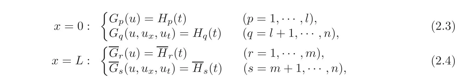
where Gp,Hp,andare all C2functions with respect to their arguments,Gq,Hq,andare all C1functions with respect to their arguments,and,without loss of generality,we may assume

In what follows,the following assumptions will be imposed totally or partially in different situations:
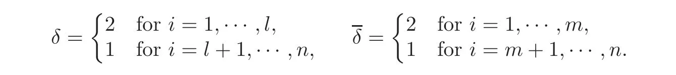
For the convenience of statement,in Case 1 we denote that
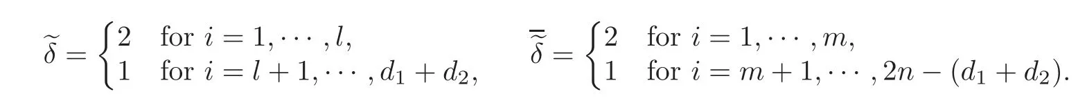
Case 2System(1.1)has d1+d2positive eigenvalues>0,>0 and 2n−(d1+d2)negative eigenvalues<0,<0(j=1,···,d1;k=d1+1,···,d2;h=d2+1,···,n),and,without loss of generality,we may assume
当汉斯·P离开时,他摆出一副正人君子的样子说:“你一定理解,我绝对不会让个人的感情来干扰我作为批评家的天良。”(2014:431)

namely,the number of positive eigenvalues is less than or equal to that of negative ones.
In this case,we prescribe the following nonlinear boundary conditions on the ends x=0 and x=L,respectively:
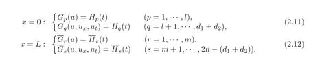
where Gp,Hp,andare all C2functions with respect to their arguments,Gq,Hq,andare all C1functions with respect to their arguments,and,without loss of generality,we may assume
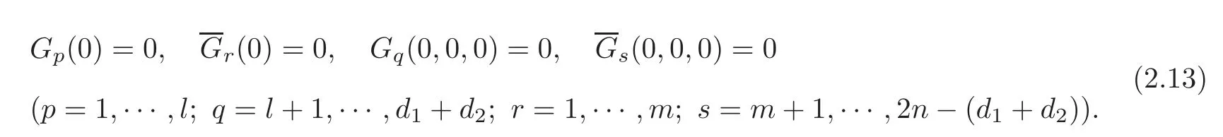
In what follows,the following assumptions will be imposed totally or partially in different situations:
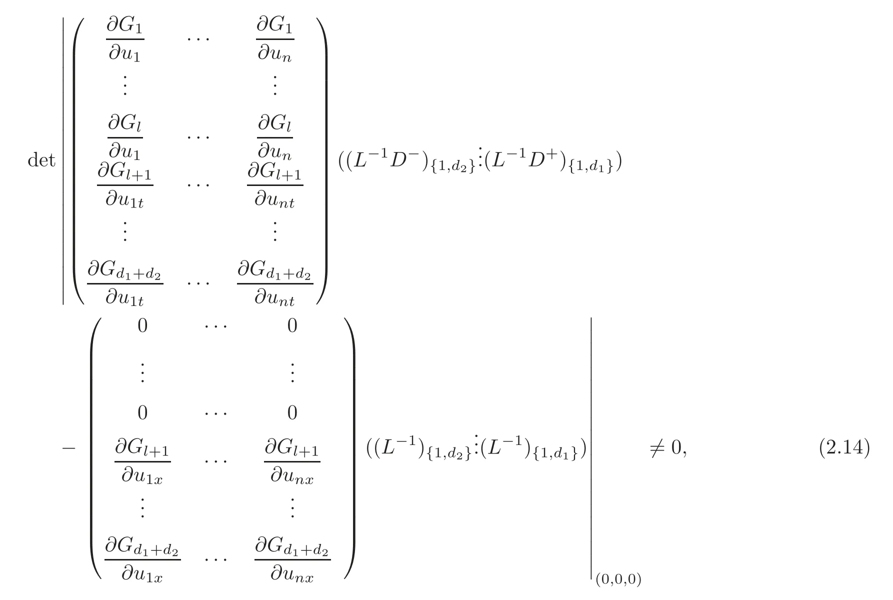
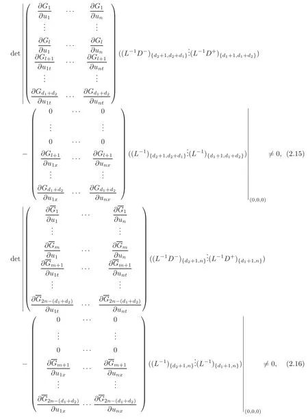
in which(L−1D−){1,d1}indicates the matrix composed of the first column to the d1th column of matrix(L−1D−),etc.
In Case 2,we denote that
Case 3System(1.1)has 2n positive eigenvalues>0(i=1,···,n).
In this case,we need only 2n boundary conditions on the end x=0:

First of all,in Case 1 we give the following lemma on the existence and uniqueness of semi-global C2solution to system(1.1)(see[14]).
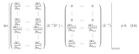
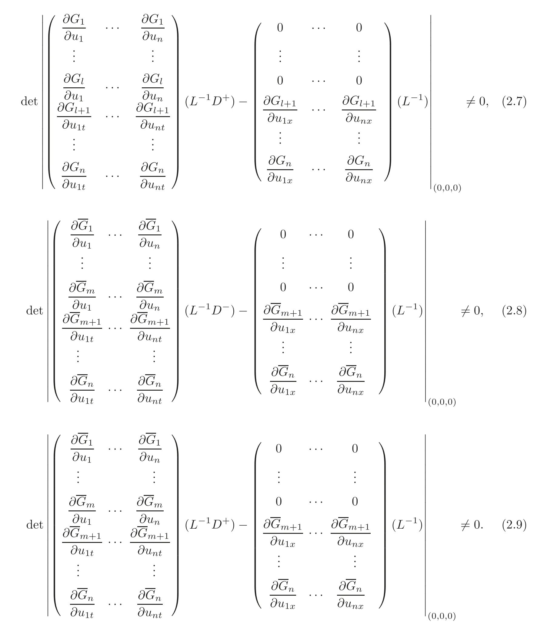
Lemma 2.1Suppose that(2.6)and(2.9)hold,and the conditions of C2compatibility are satisfied at the points(t,x)=(0,0)and(0,L),respectively.Then,for any given and possibly quite large T >0,if the norms?(ϕ,ψ)?C2[0,L]×C1[0,L],?(Hp,Hq)?C2[0,T]×C1[0,T]and(p=1,···,l;q=l+1,···,n;r=1,···,m;s=m+1,···,n)are small enough,the forward mixed initial-boundary value problem(1.1),(2.1)and(2.3)–(2.4)admits a unique semi-global C2solution u=u(t,x)on the domain R(T)={(t,x)|0≤t≤T,0≤x≤L}with small C2norm,and

where C is a positive constant.
Corollary 2.1If?(ϕ,ψ)?C2[0,L]×C1[0,L]is suitably small,then the Cauchy problem(1.1)and(2.1)admits a unique global C2solution u=u(t,x)on its whole maximum determinate domain with small C2norm,and

where C is a positive constant.
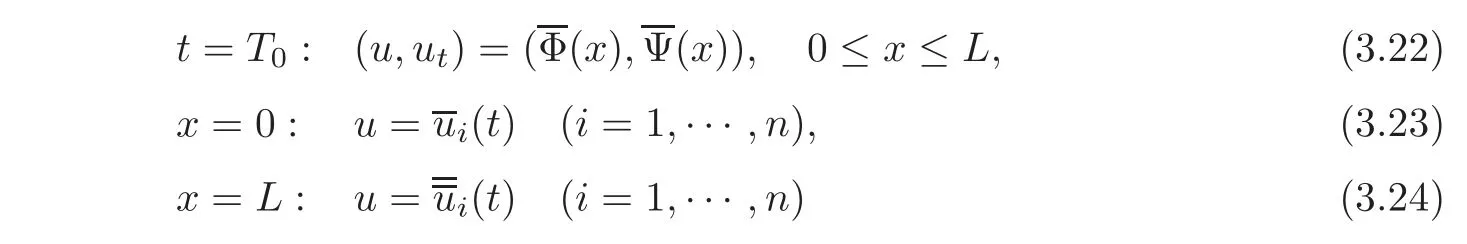
Remark 2.1If we give the following final condition

where Φ =(Φ1,···,Φn)Tis a given C2vector function,Ψ =(Ψ1,···,Ψn)Tis a given C1vector function.Suppose that(2.7)–(2.8)hold,and the conditions of C2compatibility are satisfied at the points(t,x)=(T,0)and(T,L),respectively.For any given and possibly quite large T>0,if the normsand(p=1,···,l;q=l+1,···,n;r=1,···,m;s=m+1,···,n)are small enough,the backward mixed initial-boundary value problem(1.1),(2.20)and(2.3)–(2.4)admits a unique semi-global C2solution on the domain R(T)with small C2norm,and

where C is a positive constant.
In Case 2 and Case 3,we have the corresponding existence and uniqueness of semi-global C2solution,see Lemma 2.2 and Lemma 2.3,respectively(see[14]).
Lemma 2.2Suppose that(2.14)and(2.16)hold,and the conditions of C2compatibility are satisfied at the points(t,x)=(0,0)and(0,L),respectively.Then,for any given and possibly quite large T>0,if the norms?(ϕ,ψ)?C2[0,L]×C1[0,L],?(Hp,Hq)?C2[0,T]×C1[0,T]and(p=1,···,l;q=l+1,···,d1+d2;r=1,···,m;s=m+1,···,2n−(d1+d2))are small enough,the forward mixed initial-boundary value problem(1.1),(2.1)and(2.11)–(2.12)admits a unique semi-global C2solution u=u(t,x)on the domain R(T)with small C2norm,and

where C is a positive constant.
Lemma 2.3For any given and possibly quite large T>0,if the norms

are small enough,and the conditions of C2compatibility are satisfied at the point(t,x)=(0,0),the forward mixed initial-boundary value problem(1.1),(2.1)and(2.17)admits a unique semiglobal C2solution u=u(t,x)on the domain R(T)with small C2norm,and

where C is a positive constant.
3 Local Exact Boundary Observability in Case 1
Theorem 3.1(Two-Sided Exact Boundary Observability) Suppose that aij,bij,ci,λi,μi,lij(i,j=1,···,n)are all C1functions with respect to their arguments,and(2.6)and(2.9)hold.Suppose furthermore that
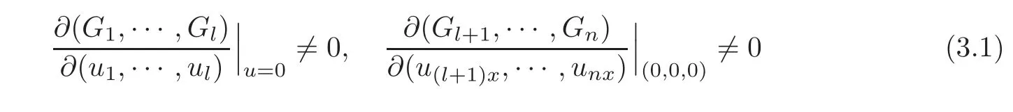
and

Let

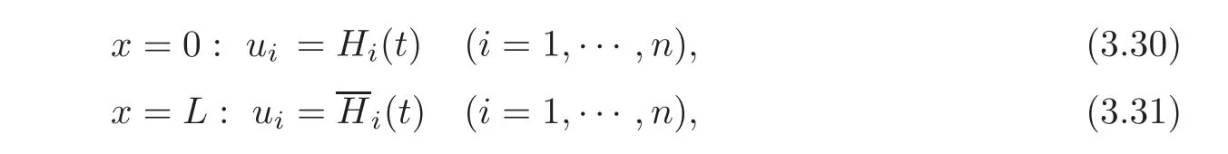
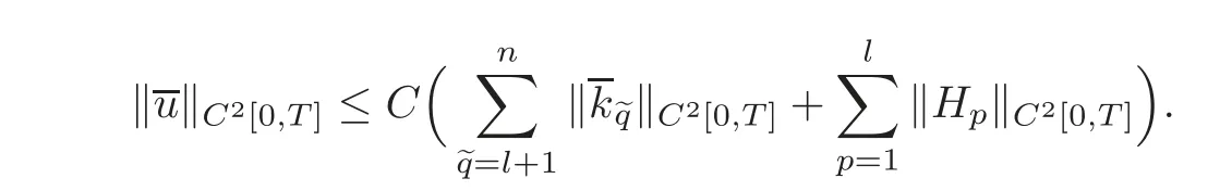
For any given initial data(ϕ(x),ψ(x))and boundary functions(H(t),H(t))with small norms?(ϕ,ψ)?C2[0,L]×C1[0,L]andsuch that the conditions of C2compatibility are satisfied at the points(t,x)=(0,0)and(0,L),respectively,if we have the observed values uq=(t),upx=(t)(p=1,···,l;q=l+1,···,n)at x=0 and us=(t),urx=(t)(r=1,···,m;s=m+1,···,n)at x=L on the interval[0,T],then the initial data(ϕ(x),ψ(x))can be uniquely determined by these observed values and(H(t),Moreover,we have the following observability inequality:
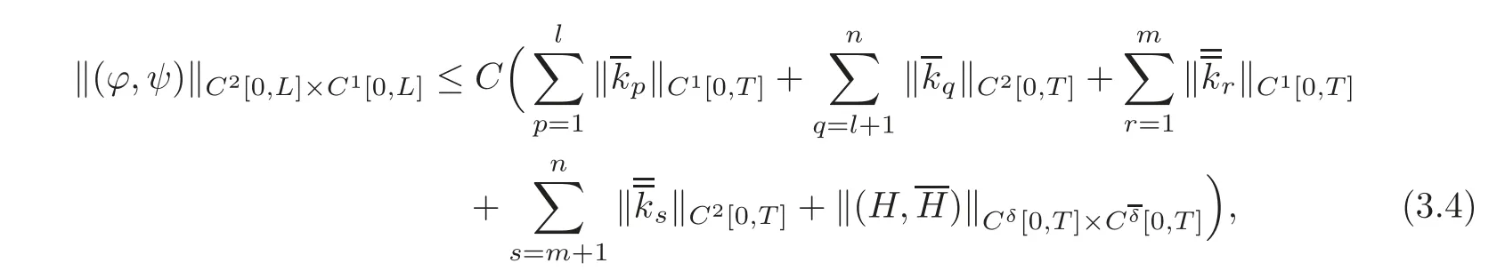
where C is a positive constant.
ProofSince?(ϕ,ψ)?C2[0,L]×C1[0,L]andare small,by Lemma 2.1,the mixed initial-boundary value problem(1.1),(2.1)and(2.3)–(2.4)admits a unique C2solution on the domain R(T)with small C2norm.Thus,the corresponding C2norms or C1norms of the observed values(p=1,···,l;q=l+1,···,n)at x=0,and(r=1,···,m;s=m+1,···,n)at x=L are all small.
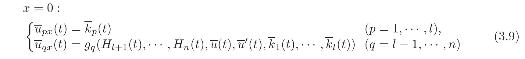
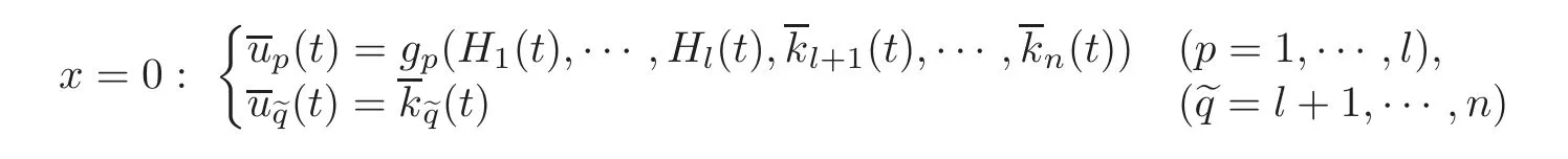
By(3.1),in a neighborhood of(u,v,w)=(0,0,0),the boundary condition(2.3)at x=0 can be equivalently rewritten as

where gp(p=1,···,l)are C2functions,gq(q=l+1,···,n)are C1functions,and by(2.5),we have

Then,the values(t)of ui(i=1,···,n)at x=0 can be uniquely determined by the observed values uq=(t)(q=l+1,···,n)at x=0 as follows:

and
On the other hand,the values(t)of uix(i=1,···,n)at x=0 can be uniquely determined by the observed values upx=(t)(p=1,···,l)at x=0 as follows:
and

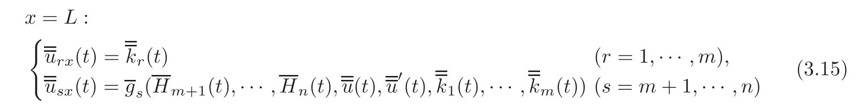
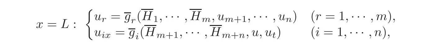
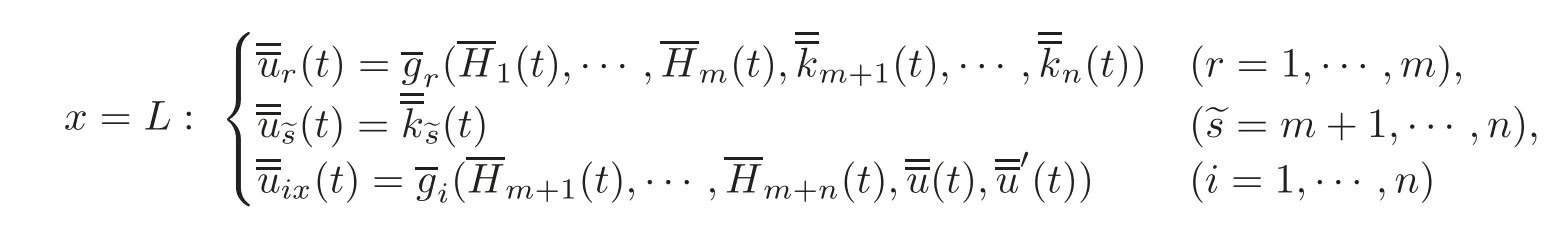
Similarly,by(3.2),in a neighborhood of(u,v,w)=(0,0,0),the boundary condition(2.4)at x=L can be equivalently rewritten as

where(r=1,···,m)are C2functions,(s=m+1,···,n)are C1functions,and by(2.5),we have

Then,the valuesof ui(i=1,···,n)at x=L can be uniquely determined by the observed values us=(s=m+1,···,n)at x=L as follows:

and

On the other hand,the valuesof uix(i=1,···,n)at x=L can be uniquely determined by the observed values urx=(r=1,···,m)at x=L as follows:
and
Changing the role of t and x,we consider the rightward Cauchy problem for system(1.1)with the initial condition

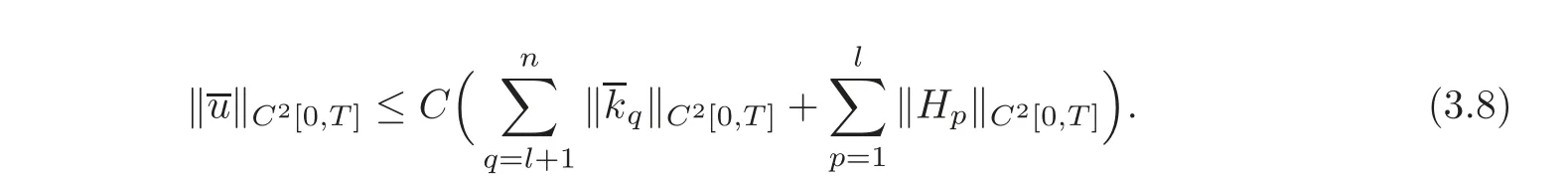
By Corollary 2.1 and noting(3.8)and(3.10),this Cauchy problem admits a unique C2solution u=(t,x)on its whole maximum determinate domain,and

Similarly,the leftward Cauchy problem for system(1.1)with the final condition

admits a unique C2solution u=(t,x)on its whole maximum determinate domain,and

Obviously,both u=(t,x)and u=(t,x)are the restrictions of the solution u=u(t,x)to the original mixed problem on the corresponding domains,respectively.
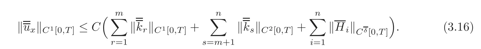
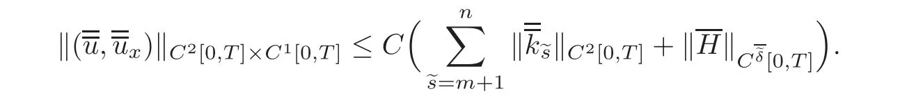
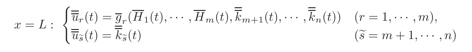
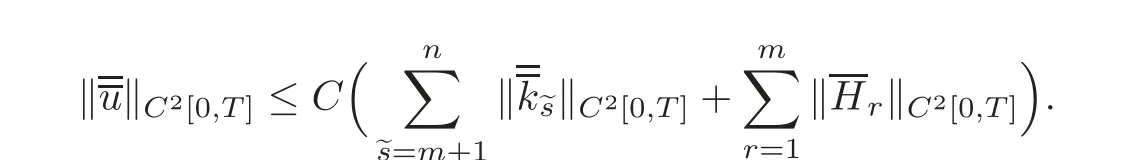
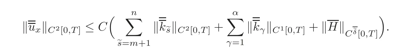
Noting(3.3),these two maximum determinate domains must intersect each other.Then,there exists T0(0 We now consider the backward mixed initial-boundary value problem for system(1.1)with on the domain R(T0)={(t,x)|0≤t≤T0,0≤x≤L}.By Remark 2.1,this backward mixed problem admits a unique C2solution u=ub(t,x),which is the restriction of the original C2solution u=u(t,x)on the domain R(T0),thus we have By(2.1)and noting(3.8),(3.14)and(3.21),we get the desired observability inequality(3.4). Theorem 3.2(One-Sided Exact Boundary Observability) Suppose that aij,bij,ci,λi,μi,lij(i,j=1,···,n)are all C1functions with respect to their arguments,and(2.6),(2.8)–(2.9)and(3.1)hold.Let For any given initial data(ϕ(x),ψ(x))and boundary functions(H(t),H(t))with small normsandsuch that the conditions of C2compatibility are satisfied at the points(t,x)=(0,0)and(0,L),respectively,if we have the observed values(p=1,···,l;q=l+1,···,n)at x=0 on the interval[0,T],then the initial data(ϕ(x),ψ(x))can be uniquely determined by these observed values andMoreover,we have the following observability inequality: where C is a positive constant. ProofChanging the role of t and x,we consider the rightward Cauchy problem for system(1.1)with the initial condition(3.17),which admits a unique C2solution u=(t,x)on its whole maximum determinate domain and(3.18)holds.Obviously,u=(t,x)is the restriction of the C2solution u=u(t,x)to the original mixed problem on the corresponding domain. Noting(3.26),this maximum determinate domain must intersect x=L.Then,there exists T0(0 We consider the backward mixed initial-boundary value problem for system(1.1)with the final condition(3.22)and boundary conditions(3.23)and(2.4)on the domain R(T0).By Remark 2.1,this backward mixed problem admits a unique C2solution u=ub(t,x)on the domain R(T0),which is just the restriction of the original C2solution u=u(t,x)on the domain R(T0),thus we have By(2.1)and noting(3.8)and(3.28),we get the desired observability inequality(3.27). Remark 3.1In Case 1,if the boundary conditions are particularly given as it is easy to see that assumptions(3.1)–(3.2)are automatically satisfied. Remark 3.2In Case 1,since the number of positive eigenvalues for system(1.1)is equal to that of negative eigenvalues,similar result holds if we take observed values at x=L instead of at x=0,and hypotheses(2.6),(2.8)–(2.9)and(3.1)are replaced by(2.6)–(2.7),(2.9)and(3.2). Let Assume that α≥0. Theorem 4.1(Two-Sided Exact Boundary Observability) Suppose that aij,bij,ci,λi,μi,lij(i,j=1,···,n)are all C1functions with respect to their arguments,and(2.10),(2.14)and(2.16)hold.Suppose furthermore that and Let For any given initial data(ϕ(x),ψ(x))and boundary functions(H(t),H(t))with small normsandsuch that the conditions of C2compatibility are satisfied at the points(t,x)=(0,0)and(0,L),respectively,if we have the observed valuesat x=0 andat x=L on the interval[0,T],then the initial data(ϕ(x),ψ(x))can be uniquely determined by these observed values and(H(t),Moreover,we have the following observability inequality: where C is a positive constant. ProofThe proof of Theorem 4.1 is similar to that of Theorem 3.1.By(4.2),in a neighborhood of(u,v,w)=(0,0,0),the boundary condition(2.11)at x=0 can be equivalently rewritten as where gp(p=1,···,l)are C2functions,gq(q=l+1,···,d1+d2)are C1functions,and by(2.13),we have Then,the values(t)of ui(i=1,···,n)at x=0 can be uniquely determined by the observed valuesat x=0 as follows: and On the other hand,the values(t)of uix(i=1,···,n)at x=0 can be uniquely determined by the observed valuesat x=0 as follows: and The observed values at x=L depend on the value of α,which is divided into two subcases. (a)α=0,namely,m=n−(d1+d2). By(4.3),in a neighborhood of(u,v,w)=(0,0,0),the boundary condition(2.12)at x=L can be equivalently rewritten as where(r=1,···,m)are C2functions,gi(i=1,···,n)are C1functions,and by(2.13),we have Then,the values(t)of uiand the values(t)of uix(i=1,···,n)at x=L can be uniquely determined by the observed values u?s=(t)(=m+1,···,n)at x=L as follows: and (b)α>0,namely,m>n−(d1+d2). By(4.3),in a neighborhood of(u,v,w)=(0,0,0),the boundary condition(2.12)at x=L can be equivalently rewritten as where(r=1,···,m)are C2functions,(β = α +1,···,n)are C1functions,and by(2.13),we have Then,the values(t)of ui(i=1,···,n)at x=L can be uniquely determined by the observed valuesat x=L as follows: and On the other hand,the values(t)of uix(i=1,···,n)at x=L can be uniquely determined by the observed valuesat x=L as follows: and The rest of the proof is similar to the proof of Theorem 3.1 and can be omitted. Similarly to Theorem 3.2,we have the following theorem. Theorem 4.2(One-Sided Exact Boundary Observability) Suppose that aij,bij,ci,λi,μi,lij(i,j=1,···,n)are all C1functions with respect to their arguments,and(2.10),(2.14)–(2.16)and(4.2)hold.Let For any given initial data(ϕ(x),ψ(x))and boundary functions(H(t),H(t))with small normssuch that the conditions of C2compatibility are satisfied at the points(t,x)=(0,0)and(0,L),respectively,if we have the observed valuesat x=0,then the initial data(ϕ(x),ψ(x))can be uniquely determined by these observed values andMoreover,we have the following observability inequality: where C is a positive constant. Remark 4.1In Case 2,suppose that the boundary conditions are particularly given as By Laplace theorem of determinant(see[15]),for the invertible matrix L(0),there exists a nonsingular subdeterminant composed of the elements of the intersections of,for instance,the first row to the d2th row with the first column to the d2th column,and we denote this d2-subdeterminant of L(0)asMeanwhile,the(n−d2)-algebraic cofactor of this d2-subdeterminant satisfiesThus it is easy to see that the assumption(4.2)is automatically satisfied.Similarly,we can also get(4.3). In Case 3,we need only to consider the local one-sided exact boundary observability at x=L. Theorem 4.3(One-Sided Exact Boundary Observability at x=L) Suppose that aij,bij,ci,λi,μi,lij(i,j=1,···,n)are all C1functions with respect to their arguments.Let For any given initial data(ϕ(x),ψ(x))and boundary functions(H(t),H(t))with small normssuch that the conditions of C2compatibility are satisfied at the point(t,x)=(0,0),if we have the observed valuesat x=L,then the initial data(ϕ(x),ψ(x))can be uniquely determined by these observed values andMoreover,we have the following observability inequality:where C is a positive constant. Comparing the observability discussed above with the controllability obtained in[14],we may find an implicit duality between the exact boundary controllability and the exact boundary observability for this kind of second-order quasilinear hyperbolic systems. For the two-sided control,we have (i)The controllability time is equal to the observability time,and both of them are sharp.The restriction on the controllability time essentially means that the two maximum determinate domains for the forward and backward Cauchy problems do not intersect each other,while,the restriction on the observability time essentially means that the two maximum determinate domains for the leftward and rightward Cauchy problems must intersect each other. (ii)Both the number of boundary controls and the number of boundary observed values are equal to 2n,which is the number of all positive eigenvalues and negative eigenvalues. For the one-sided control,we have (i)The controllability time is still equal to the observability time,and both of them are sharp.The restriction on the controllability time essentially means that the two maximum determinate domains for the forward and backward one-sided mixed problems do not intersect each other,while,the restriction on the observability time essentially means that the maximum determinate domain for the rightward Cauchy problems must intersect x=L. (ii)Both the number of boundary controls and the number of boundary observed values are equal to the maximum value between the number of positive eigenvalues and that of negative eigenvalues. [1]Guo,L.N.and Wang,Z.Q.,Exact boundary observability for nonautonomous quasilinear wave equations,J.Math.Anal.Appl.,364,2010,41–50. [2]Hu,L.,Ji,F.Q.and Wang,K.,Exact boundary controllability and observability for a coupled system of quasilinear wave equations,Chin.Ann.Math.,Ser.B,34(4),2013,479–490. [3]Li,T.T.,Exact boundary observability for 1-D quasilinear wave equations,Math.Meth.Appl.Sci.,29,2006,1543–1553. [4]Li,T.T.,Exact boundary observability for quasilinear hyperbolic systems,ESIAM:Control,Optimisation and Calculus Variations,14,2008,759–766. [5]Li,T.T.,Controllability and Observability for Quasilinear Hyperbolic Systems,AIMS Series on Applied Mathematics,Vol.3,American Institute of Mathematical Sciences&Higher Education Press,Spring field&Beijing,2010. [6]Li,T.T.and Jin,Y.,Semi-global C1solution to the mixed initial-boundary value problem for quasilinear hyperbolic systems,Chin.Ann.Math.,Ser.B,22(3),2001,325–336. [7]Li,T.T.and Rao,B.P.,Strong(weak)exact controllability and strong(weak)exact observability for quasilinear hyperbolic systems,Chin.Ann.Math.,Ser.B,31(5),2010,723–742. [8]Li,T.T.,Rao,B.P.and Wang,Z.Q.,A note on the one-side exact boundary observability for quasilinear hyperbolic systems,Georgian Math.J.,15,2008,571–580. [9]Li,T.T.and Yu,W.C.,Boundary Value Problems for Quasilinear Hyperbolic Systems,Duke Univ.Math.Ser.V,Duke Univ.Press,Durham,1985. [10]Lions,J.-L.,Exact controllability,stabilization and perturbations for distributed systems,SIAM Rev.,30,1988,1–68. [11]Lions,J.-L.,Exact Controllability,Stabilization and Perturbations for Distributed Systems(in Chinese),Vol.1,translated by Jinhai Yan and Ying Huang,Higher Education Press,Beijing,2012. [12]Russell,D.L.,Controllability and stabilization for linear partial differential equations,recent progress and open questions,SIAM Rev.,20,1978,639–739. [13]Shang,P.P.and Zhuang,K.L.,Exact observability for second order quasilinear hyperbolic equations(in Chinese),Chin.J.Engin.Math.,26,2009,618–636. [14]Wang,K.,Exact boundary controllability for a kind of second-order quasilinear hyperbolic systems,Chin.Ann.Math.,Ser.B,32(6),2011,803–822. [15]Yao,M.S.,Advanced Algebra(in Chinese),Fudan University Press,Shanghai,2005. [16]Yu,L.X.,Exact boundary observability for a kind of second order quasilinear hyperbolic systems and its applications,Nonlinear Analysis,72,2010,4452–4465. [17]Yu,L.X.,Exact boundary observability for a kind of second-order quasilinear hyperbolic system,Nonlinear Analysis,74,2011,1073–1087. [18]Zuazua,E.,Boundary observability for the space-discretization of the 1-D wave equation,C.R.Acad.Sci.Paris,Sér.I,326,1998,713–718.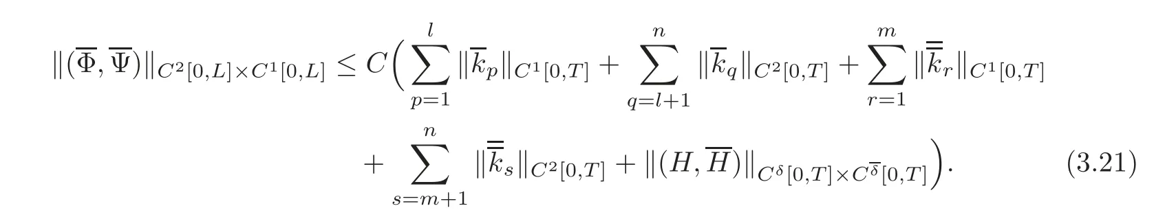


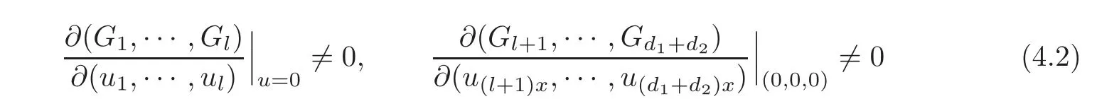
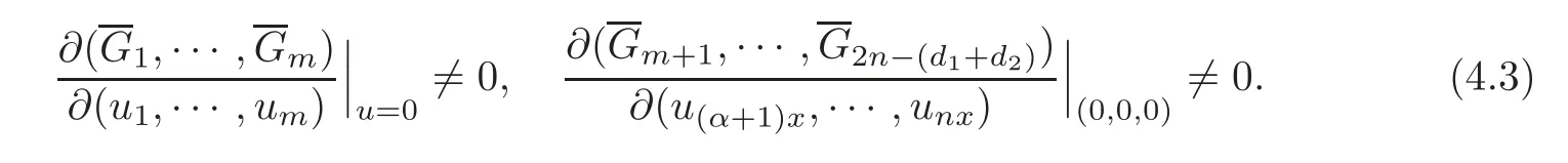
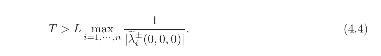
4 Local Exact Boundary Observability in Case 2 and Case 3


5 Implicit Duality Between Controllability and Observability
猜你喜欢
杂志排行

Chinese Annals of Mathematics,Series B的其它文章
- Rational Structure of X(N)over Q and Explicit Galois Action on CM Points∗
- Homogenization of Elliptic Problems with Quadratic Growth and Nonhomogenous Robin Conditions in Perforated Domains
- Asymptotic Behavior of the Incompressible Navier-Stokes Fluid with Degree of Freedom in Porous Medium∗
- Modular Invariants and Singularity Indices of Hyperelliptic Fibrations
- New Quantum MDS Code from Constacyclic Codes∗
- On Robustness of Orbit Spaces for Partially Hyperbolic Endomorphisms∗