Control of systems with sector-bounded nonlinearities:robust stability and command effort minimization by disturbance rejection
2016-05-14CarloNOVARAEnricoCANUTODonatoCARLUCCI
Carlo NOVARA,Enrico CANUTO,Donato CARLUCCI
Politecnico di Torino,Italy
1 Introduction
In this paper,the problem of controlling a system with unknown sector-bounded nonlinearities subject to external disturbances is considered.To solve this problem,we endow the control unit with a state observer,including the command-to-measurements controllable dynamics and a disturbance dynamics whose state is used to recover the unknown disturbance to reject.Observers of this kind are well known in the literature and are commonly referred to as extended state observers(ESO),disturbance observers,or unknown input observers[1–3].Extended observers are at the core of Active Disturbance Rejection Control[4,5],and of Embedded Model Control[6,7].
The most recent research in this field concerns highgain extended observers as efficient methods for feedback linearization[8].An earlier assumption on the non-linearity to be rejected was in terms of global Lipschitz continuity with respect to the state variables,as in the works of Gauthier and co-authors[9,10].Global Lipschitz continuity implies that the nonlinearity slope in the whole state space is uniformly bounded.The bound doesnotplay any role in the observerfeedback design as it is imposed to be high-gain.Since any global Lipschitz continuous function without bias(zero at the origin)is sector bounded,this latter property is assumed in the present paper.
State observers(but not extended observers)with generalized sector-bounded nonlinearities have been reported in[11].A weaker Lipschitz property(local Lipschitz continuity[12])has been assumed in the works of Khalil and co-authors[1,8],in order to include polynomial functions of arbitrary degree,whose derivative is not uniformly bounded.Of course,the observer bandwidth(BW)must be pushed to be arbitrarily large well beyond the control BW.Most of existing approaches are thus based on high gain techniques.However,these techniques may be affected by relevant problems,such as high sensitivity to measurement noise[13,14]and peaking phenomena[8].Robust stability in the presence of input nonlinearities and uncertainty has been one of the major research subjects ofActive Disturbance Rejection Control,but with somewhat different assumptions from here[3,5,15].
In this paper,we propose an alternative estimationcontrol approach,overcoming these problems.The control unit includes an ESO and a feedback law,aimed at rejecting the effects of the unknown nonlinearities and disturbances.In summary,the main novel contributions given in the paperare three.First,we derive a robuststability condition for the proposed control scheme,holding forallthe nonlinearitiesthatare bounded by a known(or estimated)maximum slope.Second,we propose an original approach,based on the asymptotes of the closed-loop transfer function(asymptotic gain design),for designing the observer and state feedback gains,allowing robust closed-loop stability and disturbance rejection.A significantresultofthe gain design is the bandwidth lower bound that,at the same time,guarantees stability and limits the gain magnitude.Third,we show that,thanks to disturbance rejection,the designed control unit is able to yield,with a minimum control effort,the same control performance as any standard statefeedback control,which on the contrary may require a“large”command activity(a similar statement appeared in[1,16]but without any formal proof).Besides robust closed-loop stability,minimum control effort is the only performance that is demanded to control design.No tracking error accuracy criterion drives the asymptotic gain design,implying that the class of the unknown disturbances and of the measurement noise does not play an explicit role in the gain design.Such a problem with its solution has been already treated in[6]and in the challenging space application of[17],by using asymptotic gain design to deal with unknown disturbances and measurement noises.By the way,the gain lower bound of the design is such to reduce the sensitivity to noise.Accuracy driven design in the presence of nonlinearities and stochastic disturbances is a subject of future developments.Two simulated examples are presented and discussed,together with accuracy indices.
The reminder of the paper is organized as follows.In Section 2,the robust control problem is formulated.In Section 3,the structure of the control unit is introduced and robust closed-loop stability conditions are derived.Section 4 develops the observer and control design methodology.In Section 5,it is shown that the proposed control strategy is able to reduce the control effortto a minimum,ensuring atthe same time a desired performance level.The simulated results are shown in Section 6.Concluding comments are given in Section 7.
2 Problem formulation
Considermstate equations indexed byj=1,...,m:
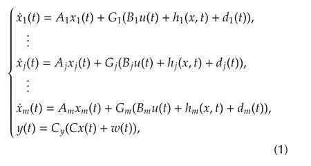
wherexj∈Rnj,nj?1,is the state vector of thejth equation,x∈Rn,n=n1+...+nm,is the total state vector,u∈Rmis the command vector,hjis an unknown function ofxto be defined below,djandw∈Rmare bounded unknown variables,y∈Rmis the output vector andCy∈Rm×Rmis an invertible matrix.As a baseline,for simplicity of notation,the initial conditions are not explicitly indicated.The matrices and vectors in(1)are
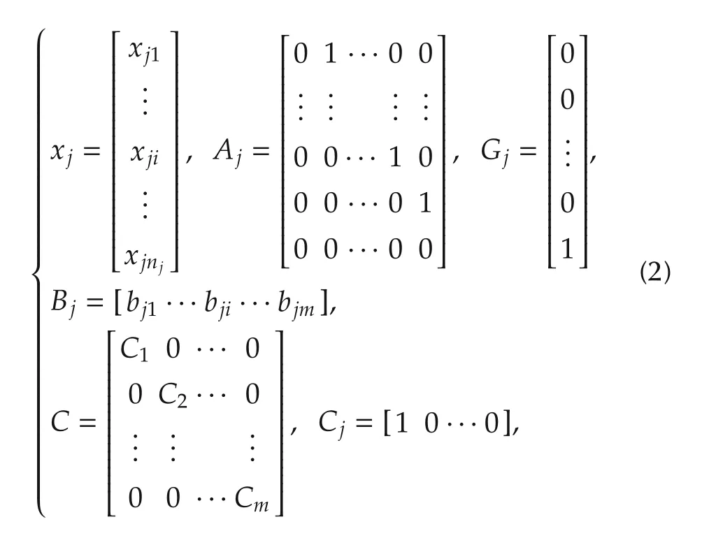
where the indexi=1,...,njrefers to a generic component ofxj.The index pairji,withj=1,...,mandi=1,...,nj,will be often replaced by the unique indexk=1,...,n,withn=n1+...+nm.Equation(1)corresponds to the MIMO normal form of feedback linearization[18].
The unknown functionhj(x,t)is assumed to be sectorbounded.That is,for anyj=1,...,mandk=1,...,n,
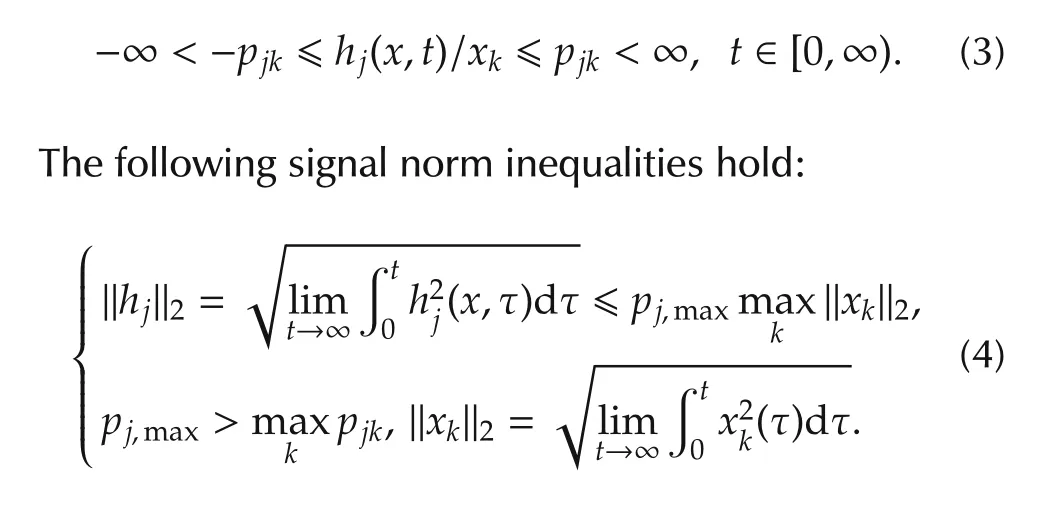
We assume that the boundpjkin(3)is unknown.Onlypj,maxis known.Note that this latter bound can be identified from experimental data either off-line or online[19].The overall bound is denoted by

Problem statementTo design a control system such that:
i)the closed-loop system is stable;
ii)the system state is regulated “close”to the origin,rejecting all the unknown disturbances and nonlinearities up to a given bandwidth,
iii)a “small”command effort is required.
The concepts of stability,disturbance rejection and command effort,here introduced in a qualitative way,will be formally defined in the paper when necessary.
Remark 1The problem of regulating the system state to zero is considered for simplicity.The control design method presented in the paper can be extended without significant modifications to the case where the state has to track a generic reference signal(the theoretical properties shown in the paper are preserved also for this more general case).
Observe that equation(1)can be rewritten in a compact form as
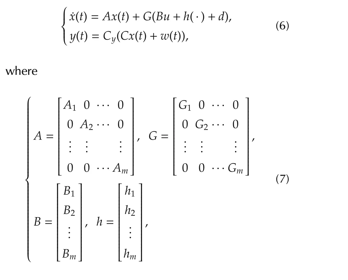
andh(·)=h(x,t).(A,G)is controllable and(C,A)is observable.The overall unknown disturbance to be estimated and rejected isdtot=h(x,t)+d.
3 Control system structure and robust stability
3.1 State observer and control law
The disturbance rejection(DR)controller that we propose is the combination of an ESO and of a control law that includes disturbance rejection.The idea behind this controller is to use the ESO to estimate both the state and the unknown nonlinearities and disturbances,and then to use a feedback law that guarantees closedloop stabilization and allows rejection of the nonlineari-ties/disturbances.The extended observer is defined by
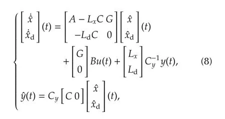
wherexd(t)∈Rmis an estimate of the unknown disturbancedtot.LxandLdare the observer gain matrices,designed in such a way that the matrix

has asymptotically stable(AS)eigenvalues.The gain matrixLx∈Rn×Rmhas the following entries,one for each state sub-vectorxjin(1),namely

andLd∈Rm×Rm.Assuming zero reference,the control law is the sum of a state feedback and of a disturbance rejection term:
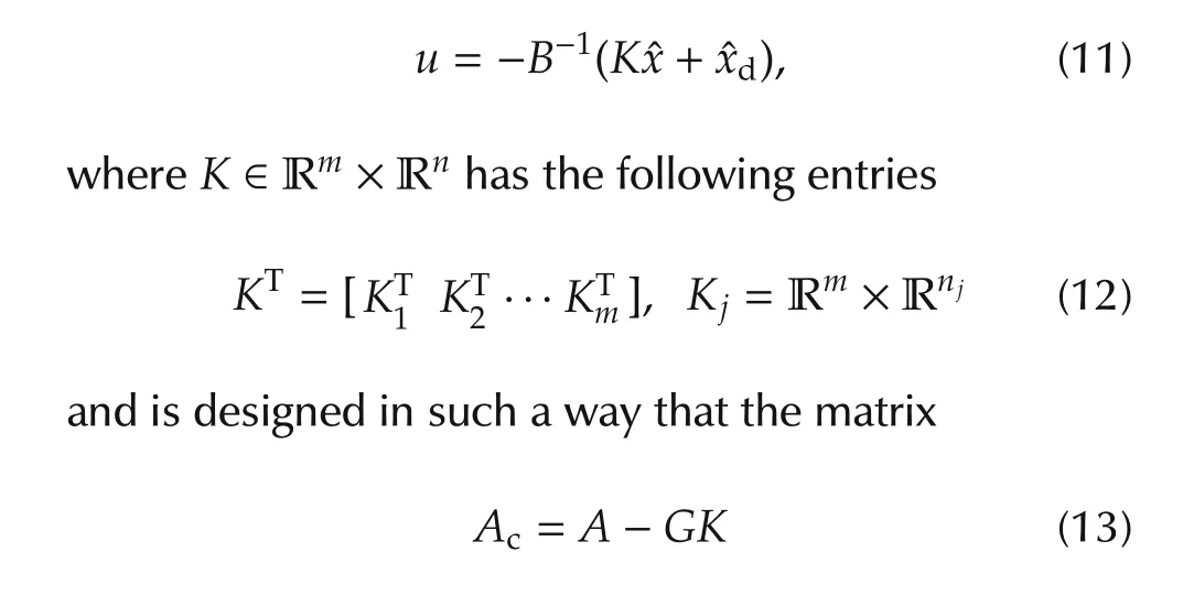
has AS eigenvalues.The following lemma is straightforward.
Lemma 1The closed-loop matrices(9)and(11)can be stabilized by decoupling the gain matrices.Thatis,Lxjis zero except on thejth column,which is denoted byLxjj,Ld=diag{Ld1,...,Ldm}is diagonal andKjis zero except on thejth row,which is denoted byKjj.The set ofthe feedback gainsis denoted withLj={Lxjj,Ldj,Kjj}.
3.2 The error equation and its transfer matrix
Stability conditions can be derived from the error equation that relatesh(x,t)tox.The estimation error

The error equation takes the form

with the following vector and matrix notations:
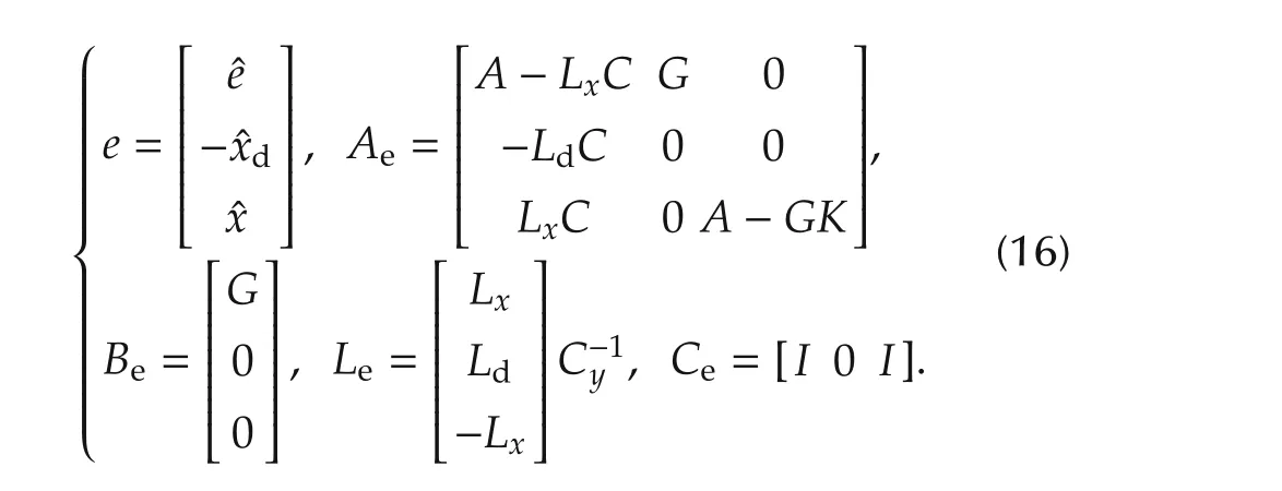
Equation(15)can be rewritten as a transfer matrix fromdtot(t)=h(x,t)+dandw(t)to the state vectorx(t):
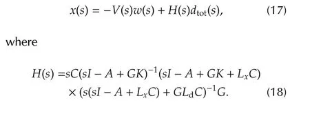
The following lemma descends from Lemma 1,if decoupled gains are adopted.
Lemma 2By assuming decoupled gain matrices as in Lemma 1,the transfer matrix in(18)becomes blockdiagonal as follows:

ProofIt is a direct consequence of Lemma 1. ?
3.3 Robust stability condition


wherewτis a truncation ofw,given by

See[8]for more details.
A stable linear system described by a transfer functionH(s)can be seen as a mapping from signals in L2eto signals in L2e.The input-output gain of this mapping is given by the H-infinity norm ofH(s),which is denoted by|H|∞.The following lemma is fundamental to derive robust stability conditions.
Lemma 3The H-infinity norms ofHji(s)andVji(s)exist and are finite.
ProofThe lemma descendsfrom the asymptotic stability of the matrixAein(16). ?
Lemma 3 implies that the linear system(15)is inputoutput stable ifh(x,t)does not depend onx.However,since in generalh(x,t)depends onx,and this makes the overall closed-loop system becomes nonlinear and possibly unstable.In this paper,we consider the following stability notion for nonlinear systems,which accounts for the effect on the system state of both input and initial conditions.
De finition 1A nonlinear system(possibly timevarying)with inputd,statexand initial conditionx0is L2eAS if:
i)Constants λ < ∞ and η < ∞ exist such that the state signal is bounded as

foranyd∈L2e;here,xanddare continuous-time signals and?·?2denotes the L2signal norm.
ii)Under a null inputd,

for any bounded initial conditionx0.
The following result provides a closed-loop stability condition for system(15)(which is equivalent to the system which consists of(1),(8)and(11)).
Theorem 1A sufficient stability condition for the system(15)is

ProofSee the appendix.
Remark 2The stability condition(24)is trobust,in the sense that it guarantees stability for all possible nonlinearitieshwhich are sector-bounded as in(3).
Remark 3According to(24),each subsystemjcan be separately designed so as to ensure stability.
4 Asymptotic gain design
In this section,we propose a novel approach for designing the gain matricesK,LxandLdin such a way that stability condition(24)is satisfied.The approach is based on the derivation of high-and lowfrequency asymptotic approximations of the transfer functions in(18).The intersections between high-and low-frequency asymptotes allow us to find gains that ensure robust stability.
4.1 Asymptotic approximations
Using the decoupled gain matrices of Lemma 1,the error equation(16)can be split intomparallel equations like in(1).These equations are only interconnected byhj(·),which in turn depends on the whole statex.The parallel equations are as follows:

wherej=1,...,m.Vectors and matrices in(25)have the same structure as in(16):
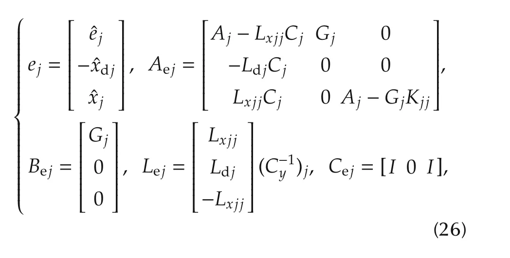


The eigenvalues of the matrixAejin(26)can be split into two separate spectra:the state observer spectrum Λpj,ofcardinalitynj+1,and the state feedback spectrumΛcj,of cardinalitynj.Thus,the eigenvalue cardinality of thejth subsystem amounts toNj=2nj+1.From(26)and(27),these eigenvalues are the roots ofthe characteristic polynomials

The notation|Λ|will be used to denote the max absolute value in Λ.The high-and low-frequency approximations ofthese transferfunctionsare given by the following theorem,which is fundamental for our design technique.
Theorem 2The high-frequency approximation ofHj(s)is

which shows that the cardinality of the zeros ofHjiamounts toMji=nj+i.The low-frequency approximation ofHji(s)is which shows thatHjipossesses onlyizeros in the origin.

ProofSee the appendix. ?
The low-frequency gainNj1in(30)can be expressed in terms of the feedback gain vectorsLxjjandKjj,and of the scalar gainLdj.
Corollary 1An alternative expression ofNj1in(30)is

ProofSee the appendix. ?
For the sake of simplicity,the state observer and the state feedback spectra Λpjand Λcjof thejth subsystem in(28)are assumed to be real and expressed in terms of only two parametersqjand γj:

where Λpjare the eigenvalues of the matrix in(9)and Λcjare the eigenvalues of the matrix in(13).Under this assumption,the following expressions of the gains in(31)is found:
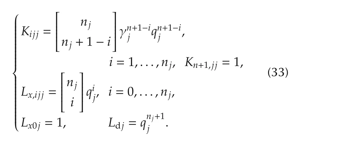
Thus,the low-frequency gainNj1becomes

The coefficient νj(γj)can be substituted by the coefficient

which has the following properties:

The last limit will be used later in our design approach.We now derive,for the generic case and for the simplified case(34),the intersection frequency ωjbetween high-and low-frequency asymptotes.
Corollary 2For anyi=1,...,nj,the magnitude of the asymptotes(29)and(30)fors=jω intersects at the angular frequency:

The magnitude at the intersection depends on the componentiand is given by

In the simplified case(34),the intersection frequency and magnitude become

ProofSee the appendix. ?
The asymptotic magnitudeHji,maxin(39)is the magnitude of the high-frequency asymptotesHj∞(s)in(29),if computed at ω =qj/νj(γj).Taking the maximum ofHji,maxwith respect toi,two different solutions can be found,depending whether the angular frequencyqj/νj(γj)is larger or smaller than unit:

Before presenting the design approach,we analyze under which conditions the magnitude|Hji|ofHji(jω)is upper bounded by low-and high-frequency asymptotes.We consider the simplified case(34)and we investigate the relative position of the poles and zeros ofHji(s).The next lemma shows that the zeros ofHji(s)and the statefeedback poles of Λcjin(28)tend to cancel each other as soon as|Λcj|tends to be larger than|Λpj|.In this case,Hji(s)tends to have onlyizeros at the origin andnj+1real poles,which implies that the magnitude|Hji(jω)|is bounded by the asymptotes in(29)and(30).
Lemma 4Let us denote withZj={-zji?0,i=1,...,nj}the set ofnjzeros ofHjiwhich are not at the origin,and refer them as the “middle”zeros.If the following limit holds

whereKjjandLx,jjhave been defined in(31)and|·|is some vector norm,thenZj→ Λcj,and theHjiremains withizeros at the origin and thenj+1 poles of Λpj.Under this condition,

ProofSee the appendix. ?
Fig.1 refers to|Hji|,withjany,nj=4,i=2 and γj={10,100}in(32).With γj=100,|Hji|is pretty bounded by the asymptotes.The low-frequency asymptote for γj=100 is not shown.
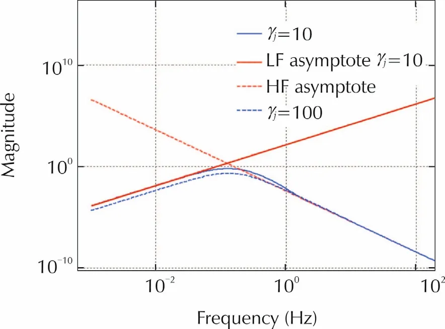
Fig.1 Magnitude Bode diagram of|H ji|and low frequency(LF)and high frequency(HF)asymptotes.The ordinate is dimensionless.
4.2 Eigenvalue placement
Lemma 4 allows us to construct an effective approach for choosing the closed-loop eigenvalues in(32)in order to satisfy the robust stability condition(24).The idea is to replace in(24)the asymptotic expressions ofHji,maxgiven by(38)and(39).Since the replacement holds for|Kjj|/|Lxjj|→ ∞,it only provides a first-trial state-observer eigenvalue-qjfor|Kjj|>|Lxjj|.Refinement can be operated either by optimizing a suitable performance functional as in the H-infinity method or by Monte Carlo runs.By replacing in(24)the expression(38)ofHji,max,the sufficient stability condition(24)changes into:
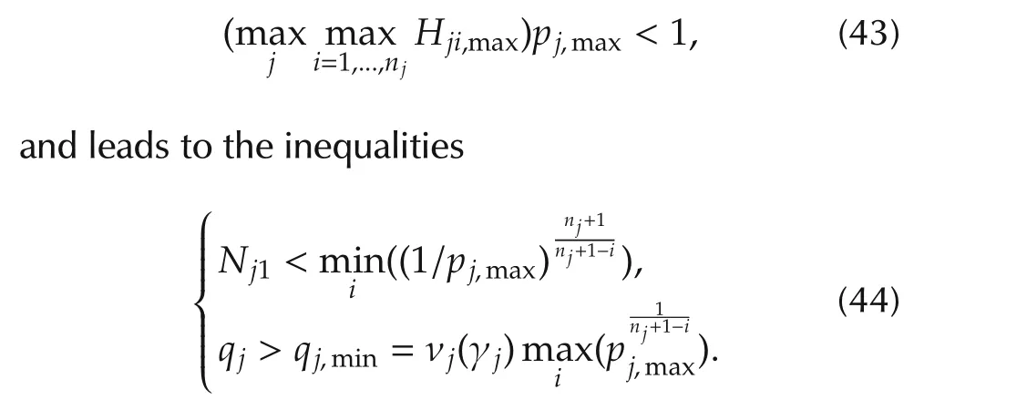

In turn,limit(36)and the second inequality in(44)lead to the inequality which is coherent with Lemma 4,as the latter demands γj→ ∞.Maximization with respect toiof(44)and(45)depends on the value ofpj,max,whether it is larger or smaller than unit.Thus,we can rewrite(44)as follows:

which is coherent with the discussion leading to(40).In practice,when the slopepj,maxis less than unit,it should be augmented top1/njj,max,in order to account fornjintegrations of the corresponding disturbance.
Theapproachthatweproposeforassigningtheclosedloop eigenvalues(32)values that satisfy the robust stability condition(24),consists in choosing the eigenvalue qjaccording to(46)andγj?1,∀j.
Remark 4Inequalities(44)and(45)are in favor of high-gain observers,since they provide a lower bound to the state observer eigenvalues.Inequality(45)shows that the minimum lower bound ofqjis obtained by a wide-band state feedback.This result is coherent with the anti-causal condition of the embedded model control[6,7],which states that,by designing a state feedback with a wider bandwidth than the state observer(in this case,γj?1),stability in the presence ofuncertainty is guaranteed by the state observer itself.
4.3 Summary of the overall design procedure
The overall DR control design procedure can be summarized as follows:
1)For each subsystemj=1,...,nin(1),with dimensionnj,the nonlinear sector boundpj,maxis estimated.
2)The separation gain γj> 1,∀j,between the state observer and,feedback law eigenvalues in(32)is chosen.This is a degree of freedom of the DR design which can be optimized in the presence of requirements other than robuststability.Forinstance,robuststability versus neglected dynamics as in[17]may be a key issue.
3)The state observereigenvalue magnitudeqj>qj,minis computed from(46).The observer and feedback eigenvalues are chosen according to(32)but,as pointed out in[17],eigenvalues should be suitably spread to reduce sensitivity overshoot.The ratioqj/qj,min>1 is dictated by other requirements than input nonlinearities,such as tracking error accuracy versus the class of unknown disturbances to be rejected and of the measurement noise.
5 Minimization of the control activity
In this section,we show that the proposed DR control method is able to yield the same control performance as any standard state feedback controller,requiring however a minimal command activity.Consider the generic control law

Suppose that this law is applied to system(6).A criterion to measure the activity of the commanduin(47)is now introduced.Sinceudepends onhand this function is unknown,the most appropriate thing we can do is to define a bound on the command amplitude,given by the following worst-case command effort(WCE):

where H is the set of all functions which are sectorbounded according to(3).As it is evident from(48),the WCE measures the performance of a controller K in terms of command activity.In the following subsections,we compare the WCE given by the DR controller with the one given by a standard worst-case state feedback strategy,and we prove an optimality result for the DR controller.For simplicity,perfect estimation is assumed for both controllers.Very similar results to the ones shown below can be obtained in the presence of estimation errors.
5.1 Standard state feedback controller
The standard pure feedback law(briefly PF)is

whereK,thathas been defined in(12),is chosen such to stabilizeAc=A-GK,andxis the system state(perfect estimation has been assumed).The other two matrices are

The standard controller uses the worst-case boundspi,maxto rejectunknown nonlinearities and disturbances.From(6),the closed-loop equation becomes

The following lemma holds.
Lemma 5The nonlinear termG(-PmaxMx/n+h(·))in(51)can be written as

whereF∈Rn×Rnis a non-positive matrix.
ProofSee the appendix. ?
Lemma 5 allows to forget the state dependence ofFand to write the free response of(51),under the assumption thatd(t)=0,as

It is now possible to bound the free response and the corresponding command signal.The norm bracket?·?applied to a matrix denotes any induced norm.
Theorem 3Under the feedback law(49),for allt?0,the free state and command responses are bounded as

ProofThe proof is straightforward. ?
5.2 Disturbance rejection controller
Consider now the control law(11),where,as for the pure feedback controller(49),we assume perfect estimation,namelyxd=h(x,t)+d(t).The control law is

and the closed-loop state equation is written as˙x(t)=Acx(t),x(0)=x0.The command and the state are now bounded as follows.
Theorem 4With the feedback law(55),for allt?0,the free state and command responses are bounded as

where the matrixP∈Rm×Rncontains all the bounds defined in(3).
ProofIt is a direct consequence of(6)and(55). ?The norm ratio
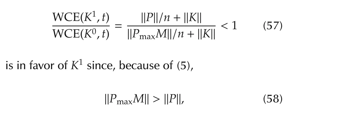
and the left hand side of(57)tends to unit if and only if some entry ofKtends to infinity.
Inequalities(57)and(58),together with Theorems 3 and 4,show that the proposed disturbance rejection(DR)controller is able to yield the same control performance(in terms of speed of response)as any standard state feedback controller,by requiring however a reduced(worst-case)command effort.The advantage is due to the fact that the command activity of the DR controller is just the one needed to reject the effect of nonlinearities and disturbances,nothing less,nothing more.On the contrary,a standard controller provides a command dealing with the worst-case nonlinearities and disturbances,and thus its activity may be significantly larger than the one of the DR controller.
An even more general result can now be proved.The DR controller,given a fixed performance level,requires the minimum command activity among all the controllers defined by a control law of the form

The first term on the right hand side of(59)is a state feedback and the second term is a sector-bounded timevarying command which compensates the effects of unknown nonlinearities and disturbances.
Theorem 5Consider the controllerK1defined by the feedback law(55).Then,for allt?0,

whereAc=A-GKand KSTV denotes the set of all the controllers defined by a feedback law of the form(59),with a fixed gain matrixK.
ProofSee the appendix. ?
6 Simulated results
In this section,two examples are presente d.They aim to outline the design methodology of the previous sections.In both examples,control strategies are implemented in continuous time and no measurement noise is considered.
6.1 Example 1
The first case is a multivariate equation like(1)withm=2,n1=1,n2=2 andn=3.The state equation matrices are

The unknown state–dependent disturbance functions are assumed to be nonlinear in their coefficients and sector-bounded.They are written as

whereHjk(t)and τjk(t)are time varying bounded functions.The slopes of the functionsh22(x2)andh23(x3)shown in Fig.2 are reconstructed from simulation.Each subsystem is also affected by a bounded stochastic disturbancedjhaving a cutoff polepdj=-0.2 rad/s,j=1,2.
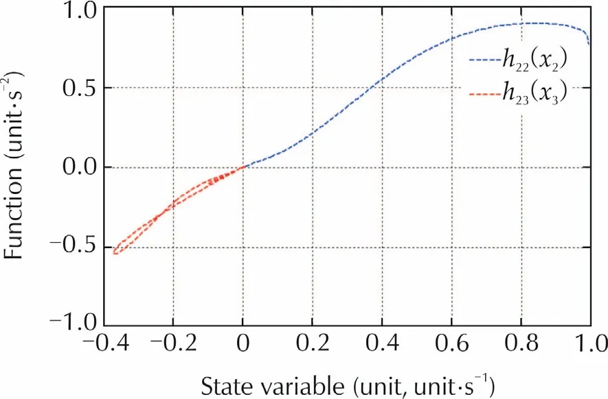
Fig.2 Simulated nonlinear functions.The abscissa x2 has arbitrary units.The abscissa x3 is given in unit/s.The ordinate is given in unit/s2.
The unknown boundspj,maxare estimated from

The matrixAin(61),if filled with the signed sector bounds in(63),is unstable.The decoupled state observers in(8)(second and third order)are designed by assuming equal eigenvalues λpk?-4p0?-20 rad/s,k=1,...,n+2.These values are the result of the upper inequality in(46)since,from(63),pmax>1 holds.Assuming γj=1 in(32)(i.e.,the same eigenvalues for state observer and feedback law),the upper inequality in(46)becomes

The decoupled state feedback eigenvaluesλck,k=1,2,3(first and second order)are taken equal and varied in the range-0.25÷-32 rad/s so as to verify(57).The absolute range goes from the disturbance cutoff pole|pd|to above the state observer pole 2pmax.The standard state feedback is implemented as in(49),whereKis the same as the disturbance rejection controller in(55),and the knownpmaxin(54)ispmax?p.The state variable of the standard state feedback are provided by an output filter,whose bandwidth is sufficiently wide not alter the state feedback eigenvalues.Initial states arex1(0)=x2(0)=1,x3(0)=-0.1 rad/s.
The output and command time profiles and their norms(the max absolute value and the RMS)are taken as performance variables.
The simulated ratio(57)ofu2,which is the command of thej=2 subsystem(second order),is plotted in Fig.3.As predicted by(57),the ratio tends to unit for increasing eigenvalues.Fig.3 shows also the RMS ratio ofy2after the initial transient whose duration depends on the state feedback eigenvalues.The ratio is in favor of the DR controller.
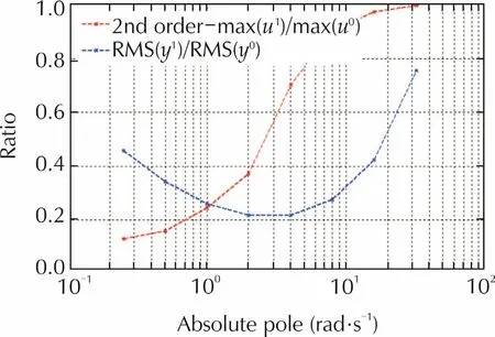
Fig.3 Command and output ratio for j=2.
Fig.4 shows the RMS ratio of the steady-state outputy2(after the initial transient)and the RMS of the DR response.The ratio is an accuracy index,and the minimal value in the presence of measurements noise is very close topmax/2=5 rad/s.The ratio varies with the measurement noise variance but this proves that the asymptotic gain design can be extended to include accuracy as a performance index.In the absence of measurement noise,the ratio converges to zero as soon as the state feedback poles tend to infinity,which corresponds to the anti-causal limit in[7].
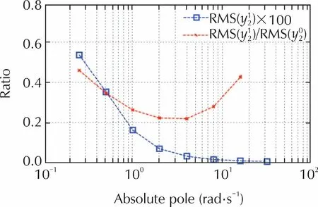
Fig.4 RMS of the steady-state output y2.
Fig.5 shows the transient response ofy1(first order subsystem)under pure feedback(solid line)and DR controllers(dashed lines).The DR response looks more regular and the initial command about one third of the pure-feedback command,as expected.
Fig.6 shows the steady-state response of the outputy2which is dominated by the stochastic disturbance.Also in this case,DR controller performs much better than the pure state feedback especially for what concerns accuracy,which is in agreement with the bottom curve in Fig.3.
A peculiar feature of the DR controller is to reduce to a minimum the feedback command effort,once the initial state has been brought to the reference value.The subject is not treated in this paper,but Fig.7 agrees with this statement.
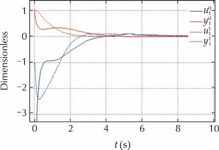
Fig.5 Transient response of the output y1.
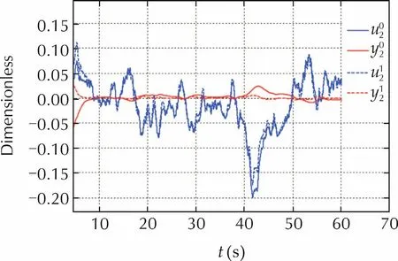
Fig.6 Steady response of the output y2.
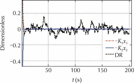
Fig.7 DR command components.
6.2 Example 2
In the second example,we consider the problem of controlling the nonlinear system in[20],whose state equations are:

where θ1=-2,θ2=1,θ3=0.5,θ4=1,θ5=-2,θ6=1,d(t)=sint,and ω is the state of the neglected dynamics

Here,dωis a zero-mean wide-band Gaussian noise with variance σ2d=400.First,a bound on the slope of the nonlinearity in(64)is estimated from simulations involving trajectories in a “large”domain of the state space.The boundp1max(to be treated as unknown in control design)is equal to Then,by fixing γ1=1/2 andv1(γ1)?2.3,after some small adjustments,the decoupled state observer(8)is designed by choosing eigenvalues as{q1=-49,q2=-51,q3=-48}rad/s.The decoupled state feedback controller is designed by choosing half magnitude eigenvalues{-24,-22}rad/s,since γ1=1/2.

For comparison,a standard state feedback controller is implemented as in(49).The true state has been replaced by the estimated state,using the same state observerdesigned forthe DRcontroller.The state feedback gainKis the same as the DR controller,andpmaxin(54)is set equal topmax?p1,max.
A Monte Carlo simulation with 100 trials is carried out.The initial state conditions are randomly selected in the interval[-2,2].The performance indexes are chosen to be the max absolute value and the RMS of the output and command time profiles.The average values of these indexes obtained by Monte Carlo trials are reported in Table 1,together with the output settling time(defined as the time interval where the output absolute value decreases below 0.01).Time profiles of the state variables in the case of the DR controller are shown in Fig.8.They refer to a single trial with initial conditions close to unit.The time profiles of the true nonlinear termhand of the predictedxdare shown in Fig.9.
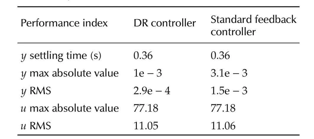
Table 1 Average control performance indexes obtained by Monte Carlo trials.
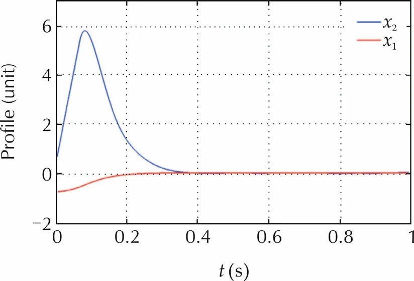
Fig.8 Time profiles of the state variables under DR controller.
The above results allow to conclude that the two controllers require almost the same command activity but the DR controllerisable to achieve a betterperformance.Note that the nonlinearity in(64)is sector-bounded on every compactsubsetofthe state space butis notsectorbounded on the whole state space.This implies that the stability sufficient condition(24)holds for all the state trajectories contained in a compact set where the nonlinearity slope is bounded by the estimated valuep1max,which bound does not hold in the whole state space.The issue can be easily overcome by estimatingp1maxby means of simulated trajectories which explore a sufficiently large subset of the state space.This point is quite important since it shows that the proposed DR control design approach can be applied to situations where the nonlinearity in(3)is sector-bounded only in a compact set.
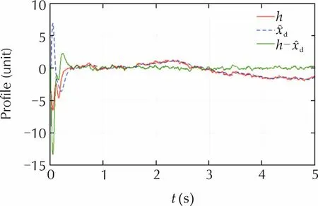
Fig.9 Time profile of the true and predicted nonlinear terms.
7 Conclusions
The paper proves a small-gain stability theorem for a multivariate dynamic system subject to unknown state dependent disturbances that are sector-bounded.Stability and performance are guaranteed by a disturbance rejection controller.A lowerbound to the extended state observer eigenvalues is derived using asymptotic transfer functions.The control effort of the DR controller is compared with a standard robust controller and the DR controller is proved to demand a minimum command effort.Further developments concern the extension to nonlinearities that are only locally Lipschitz bounded and the assessment of the accuracy performance.
[1]L.B.Freidovich,H.K.Khalil.Robust feedback linearization using extended high-gain observers.Proceedings of the 45th IEEE Conference on Decision and Control,San Diego:IEEE,2006:983–988.
[2]A.Radke,Z.Gao.A survey of state and disturbance observers for practitioners.Proceedings of the American Control Conference,Minneapolis:IEEE,2006:2209–2214.
[3]B.Guo,Z.Zhao.On convergence of non-linear extended state observer for multi-input multi-output systems with uncertainty.IET Control Theory&Applications,2012,6(15):2375–2386.
[4]Z.Gao.On the centrality of disturbance rejection in automatic control.ISA Transactions,2014,53(4):850–857.
[5]J.Li,Y.Xia,X.Qi,et al.Absolute stability analysis of nonlinear active disturbance rejection control for single-input–singleoutput systems via the circle criterion method.IET Control Theory&Applications,2015,9(15):2320–2329.
[6]E.Canuto,W.A.Bravo,A.Molano,etal.Embedded modelcontrol calls for disturbance modeling and rejection.ISA Transactions,2012,51(5):584–595.
[7]E.Canuto.Embedded model control:outline of the theory.ISA Transactions,2007,46(3):363–377.
[8]H.K.Khalil.High-gain observers in nonlinear feedback control.International Conference on Control,Automation and Systems,Seoul:IEEE,2008:13–23.
[9]G.Besan¸con.High-gain observation with disturbance attenuation and application to robust fault detection.Automatica,2003,39(6):1095–1102.
[10]J.P.Gauthier,H.Hammouri,S.Othman.A simple observer for nonlinear systems application to bioreactors.IEEE Transactions on Automatic Control,1992,37(6):875–880.
[11]K.Vijayaraghavan.Observer design for generalized sectorbounded noisy nonlinear systems.Proceedings of the Institution of Mechanical Engineers–Part I:Journal of Systems and Control Engineering,2014,228(9):645–657.
[12]H.K.Khalil.Nonlinear Systems.2nd ed.Upper Saddle River:Prentice-Hall,1996.
[13]J.H.Ahrens,H.K.Khalil.High-gain observers in the presence of measurement noise:a switched-gain approach.Automatica,2009,45(4):936–943.
[14]A.A.Prasov,H.K.Khalil.A nonlinear high-gain observer with measurement noise in a feedback control framework.IEEE Transactions on Automatic Control,2013,58(3):569–580.
[15]Q.Zheng,L.Gao,Z.Gao.On stability analysis of active disturbance rejection control for nonlinear time-varying plants with unknown dynamics.Proceedingsofthe46thIEEEConference on Decision and Control,New Orleans:IEEE,2007:3501–3506.
[16]S.Kwon,W.K.Chung.A robust tracking controller design with hierarchical perturbation compensation.Journal of Dynamic Systems Measurement and Control,2002,124(2):261–271.
[17]E.Canuto,L.Colangelo,M.Lotufo,et al.Satellite-to-satellite attitude control of a long-distance spacecraft formation for the next generation gravity mission.European Journal of Control,2015,25:1–16.
[18]S.Sastry.Nonlinear Systems:Analysis,Stability,and Control.New York:Springer,1999.
[19]M.Milanese,C.Novara.Unified Set Membership theory for identification,prediction and filtering of nonlinear systems.Automatica,2011,47(10):2141–2151.
[20]Z.Zhang,S.Xu.Observer design for uncertain nonlinear systems with unmodeled dynamics.Automatica,2015,51:80–84.
Appendix
Proof of Theorem 1From Lemmas 1 and 3,it follows that the signalxjis bounded as

wherej=1,...,m,i=1,...njandzis the free response of the linear system(15).Thus,from(4),it follows that

wherek=1,...,n.Taking the maximum overk=ji,we obtain
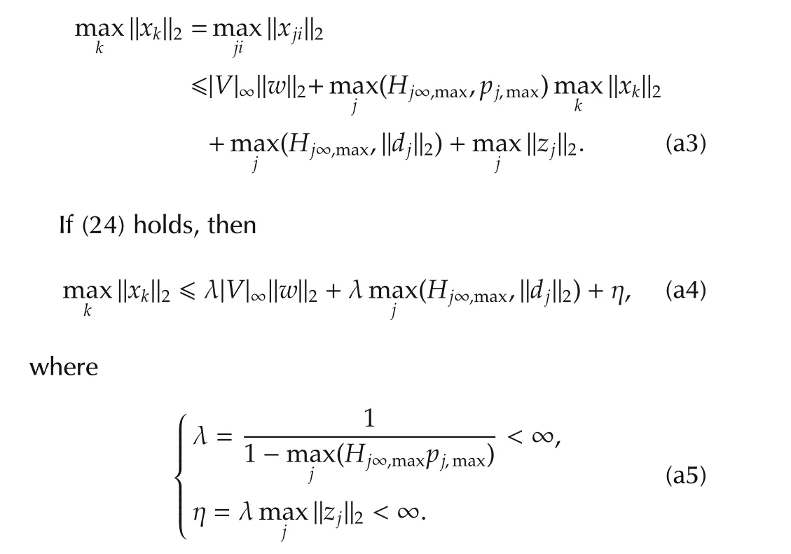
In(a5)?zj?2is bounded since it is the free response of an AS linear system.L2easymptotic stability follows from(a4)and from the fact that,for nullwandd,zj(t)converges to 0 ast→ ∞. ?


The sequence proves(30)and that onlyizeros lie in the origin. ?
Proof of Corollary 1We start from equation(30)and we compute the inverse ofAejas follows:

where the notations below have been employed
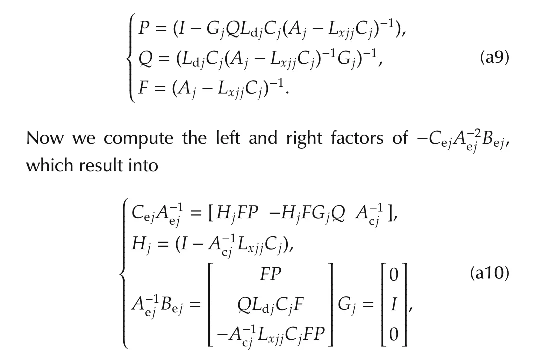
since the following equalities hold

As a first result,the right factor in(30)holds

Now,the left multiplication of(a12)times[1 0 ···0]yields

and proves that the right factor in(a12)holds
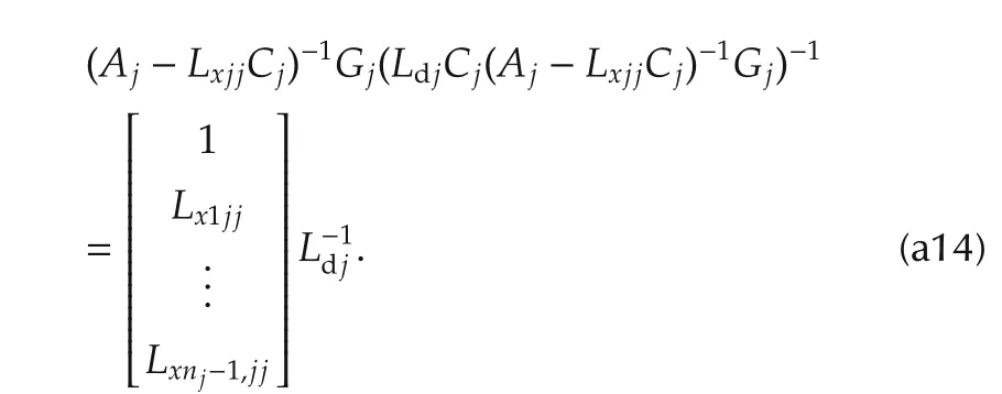
Multiplication of(a13)times(a14)provides(31). ?
Proof of Corollary 2The asymptotic equality|Hji∞(jω)|=|Hji0(jω)|between(29)and(30)can be rewritten as

and immediately yields(37),which does not depend on the componenti.The magnitude in(38)follows by replacing(37)either into|Hji∞(jω)|or into|Hji0(jω)|.Frequency and magnitude in(39)follows by substitutingNjiwith the expression in(34). ?
Proof of Lemma 4The polynomial of middle zeros ofHjiholds
The generic coefficient in(a16)can be written as a function of the coefficients κm(Lkxjj/Khjj),which are linear combinations of the ratiosLkxjj/Khjjbetween the entries ofLxjjandKjj,and converge to zero as soon as|Kjj|/|Lxjj|→∞.Thus the following expression and limit

imply thatZj→ Λcj.Inequalities in(42)are justified by the zeros ofHjibeing concentrated at the origin. ?
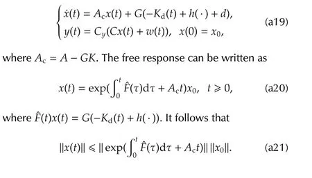
Proof of Lemma 5Fis a row-block matrix,whosejth blockFjis zero except for thenjth row.Using(3),thekth column of this row is non-positive as shown by

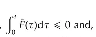
Proof of Theorem 5Assuming the control law(59),the closed-loop equation of(6)becomes
杂志排行
Control Theory and Technology的其它文章
- Extended state observer for uncertain lower triangular nonlinear systems subject to stochastic disturbance
- Sampled-data extended state observer for uncertain nonlinear systems
- On ADRC for non-minimum phase systems:canonical form selection and stability conditions
- Robust flat filtering DSP based control of the boost converter
- Yet another tutorial of disturbance observer:robust stabilization and recovery of nominal performance
- Active disturbance rejection control:between the formulation in time and the understanding in frequency
