Variable selection in identification of a high dimensional nonlinear non-parametric system

Er-Wei BAI,Wenxiao ZHAO ,Weixing ZHENG

1.Department of Electrical and Computer Engineering,University of Iowa,Iowa City,Iowa 52242,U.S.A.;

2.School of Electronics,Electrical Engineering and Computer Science,Queen’s University,Belfast,U.K.;

3.Key Laboratory of Systems and Control,Academy of Mathematics and Systems Science,National Center for Mathematics and Interdisciplinary

Sciences,Chinese Academy of Sciences,Beijing 100190,China;

4.School of Computing,Engineering and Mathematics,University of Western Sydney,Penrith NSW 2751,Australia

Received 16 January 2015;revised 26 January 2015;accepted 28 January 2015

Variable selection in identification of a high dimensional nonlinear non-parametric system

Er-Wei BAI1,2†,Wenxiao ZHAO3,Weixing ZHENG4

1.Department of Electrical and Computer Engineering,University of Iowa,Iowa City,Iowa 52242,U.S.A.;

2.School of Electronics,Electrical Engineering and Computer Science,Queen’s University,Belfast,U.K.;

3.Key Laboratory of Systems and Control,Academy of Mathematics and Systems Science,National Center for Mathematics and Interdisciplinary

Sciences,Chinese Academy of Sciences,Beijing 100190,China;

4.School of Computing,Engineering and Mathematics,University of Western Sydney,Penrith NSW 2751,Australia

Received 16 January 2015;revised 26 January 2015;accepted 28 January 2015

The problem ofvariable selection in system identification ofa high dimensionalnonlinearnon-parametric system is described.The inherent difficulty,the curse of dimensionality,is introduced.Then its connections to various topics and research areas are briefly discussed,including order determination,pattern recognition,data mining,machine learning,statistical regression and manifold embedding.Finally,some results of variable selection in system identification in the recent literature are presented.

System identification,variable selection,nonlinear non-parametric system,curse of dimensionality

DOI 10.1007/s11768-015-5010-9

1 Problem statement

Considers a stable scalar discrete nonlinear nonparametric system

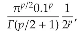
This implies that in a practical situation,the required data lengthNis gigantic even for a modestp.The curse of dimensionality is a fundamental problem for all local average approachesin many fields,notlimited to system identification.

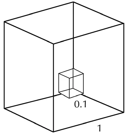
Fig.1 Illustration of empty space in a three dimensional space.

Notation used in this paperisstandard.(Ω,F,P)represents a basic probability space and ω is an element in Ω.Denote byMthe 2-norm of a matrixM.Denote byν(·)varthe total variation norm of a signed measure ν(·).The invariant probability measure and density of a Markov chain are represented byPIV(·)andfIV(·),respectively,if they exist.Denote byf(·)the gradient of a functionf(·).sgnxstands for the sign function,

2 Variable selection

For many practical applications,however,systems are sparse in the sense that not all variablesxi(k)’s,i=1,2,...,pcontribute to the outputy(k)or contribute little or are dependent.If those variablesxi(k)’s that do not contribute or are dependent can be identified and removed,then the dimension involved for identification could be much smaller.This is referred to as the variable selection problem in the literature and is a critical step for nonlinear non-parametric system identification if the dimensional is high and the data set is not big.

3 Linear vs nonlinear

Despite its importance,there are only scattered efforts for variable selection in a nonlinear non-parametric setting.There is a substantial difference between a linear setting and a nonlinear setting besides nonlinearity.Variable selection in a linear setting is a global concept,and when we say that a variable contributes,it contributes globally independent of the operating point.In contrast,whether a variable contributes or not in a nonlinear setting could be a local concept depending on the operating range.For example,let

whereQis certain region.Obviously,xp(k)contributes outside the RegionQbut does not contribute inside the RegionQ.

Also it is important to note that a number of methods developed in a linear setting do not work in a nonlinear setting and often provide misleading information.One example is the powerful correlation method[4–6].For instance,lety(k)=x(k)·1,wherex(k)’s are iid and uniformly distributed in[−1,1].It is easy to verify that the correlation coefficient ofxandyis 1 as expected.Now lety(k)=x(k)2·1.The correlation coefficient is 0 despite the fact thatyis a deterministic function ofxas shown in Fig.2.

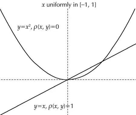
Fig.2 Nonlinear correlation.

4 Connections to other areas and discussions

Though our focus here is on system identification,the problem is similar in several other fields.For instance,the same problemy=f(x)+voccurs in patter recognition wherexandyare referred to as data and pattern,respectively,in data mining referred to as feature and label,in machine learning referred to as input and target and in statistics referred to as input and trend,as demonstrated in Fig.3.There exists a large volume of work reported in the literature of those fields,and some ideas are useful for system identification purposes.

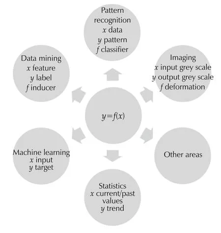
Fig.3 Connection to other areas.

4.1 Order determination

Variable selection is closely related to order determination of a nonlinear system in the literature.For instance,given a nonlinear autoregressive system with exogenous input(NARX),the order determination is to find the minimumlso that the system can be written asy(k)=f(y(k−1),...,y(k−l),u(k−1),...,u(k−l)).In otherwords,once the orderlis determined,all variablesy(k−i),u(k−i),ilare assumed to be the contributing variables and all variablesy(k−i),u(k−i),igt;lare the non-contributing ones.The order determination has been frequently used as a tool for variable selections in the literature,e.g.,in a neural network setting[7]or in a NARX setting[8,9].There are also a couples of variants of order determination reported in the literature.One is by the Gaussian regression model[10]and the other is the false nearest neighbor[11–14].Obviously,order determination is not variable selection.In fact,variable selection goes further than order determination.Even in a setting of the NARX system with a determined orderl,some of variablesy(k−i),u(k−j),i,jlmay still not contribute and could be removed by variable selection,but this is not a concern of the order determination.

4.2 Projection to a lowerdimensionalspace ormanifold

Variable selections can be carried out basically in two ways,with or without the involvement of the output values,referred to as supervised or unsupervised learning.Define

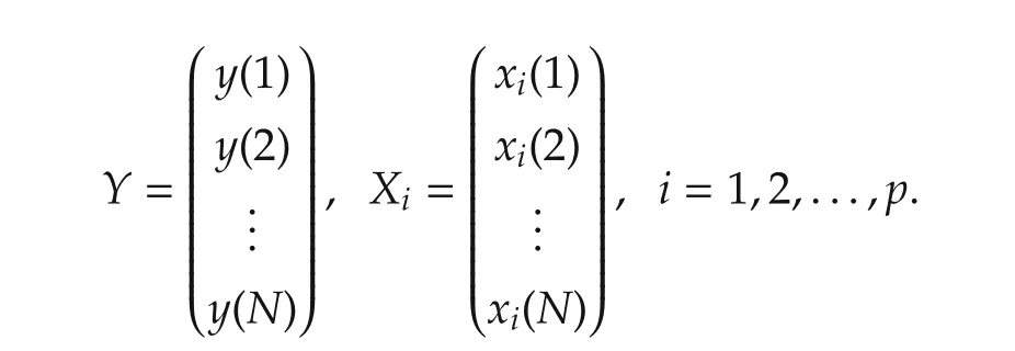
The unsupervised learning is undertaken by checking the regressorvectorstructure(X1,...,Xp).Suppose thatX1,...,Xpare in a subspace or lie on a low dimensional manifold.Then there exist a known or unknownqlt;pand some known or unknown functionsgand¯fsuch that

which implies

thereby resulting in a low dimensional(p−q)system.A special case is that(X1,...,Xp)is in a linear subspace.In such a case,by checking the rank of the regressor matrix(X1,...,Xp),one can easily determine how many regressor vectors are linearly independent,say(p−q).Then,it is trivial to calculate

for a(p−q)×NmatrixAand this in turn results in

Though much more work is involved,the same idea applies when(X1,...,Xp)lies on a low dimensional manifold.

4.3 Hard and soft approaches

Of course,a critical step for any soft approach is the definition of what constitutes an insignificant contribution and a way to test it.In summary,the ambient dimension could be very high,yet its desired properties are embedded in or very close to a low dimensional manifold.The goal here is to design efficient algorithms that reveal dominant variables for which one can have some theoretical guarantees.

4.4 Manifold embedding

In(2),what constitutes an approximation deserves more discussion because different meanings imply different results and algorithms.A very common theme in manifold embedding is to preserve local distance or structure.There are a number of different algorithms but many can be traced back to multidimensional scaling[14]and locally linear embedding[15].In locally linear embedding,one first tries to find a local structure by representingx(i)in terms ofx(j)’s in the following way:

where the coefficientswijdetermine the local structure.Then,letz(i)∈Rqbe a low dimensionalvectorsatisfying

The key idea is to find a lower dimensionalz(i)∈Rq,i=1,2,...,Nfor replacingx(i)∈Rp,i=1,2,...,Nthat resembles the local structure ofx.Finally,one hasy=f(x)≈f(z).

In multidimensional scaling[14],a distance is defined by

4.5 Johnson-Lindenstrauss theorem

Johnson-Lindenstrauss theorem[16]states that if the pairwise Euclidean distance is of concern,then any set ofkpoints in ap-dimensional space can be embedded into aqO(?−2log(k))dimensionalspace,independent ofp,i.e.,for some matrixQ:Rp→Rqand?∈(0,1/2)such that,with a high probability

In other words,if pairwise Euclidean distance is of interest,then the space is approximatelyqdimensional instead ofpdimensional,as illustrated in Fig.4.

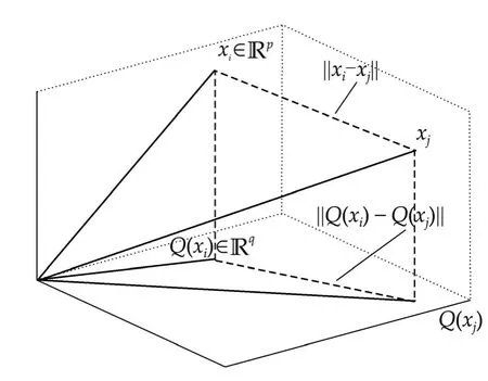
Fig.4 Illustration of Johnson-Lindenstrauss result.

4.6 Supervised and unsupervised learning

The ideas of locally linear embedding,multidimensional scaling and many others in machine learning are unsupervised training which project data to a lower dimensional manifold based on some local features while ignoring the output variabley.Note that in system identification,the output error is one of the major concerns,and ignoring the output values and checking the structure of the regressor matrix alone do not always solve the variable selection problem[17].For example,if(X1,...,Xp)are linearly independent and in fact do not lie on any low dimensional manifold butfdoes not depend on(Xi1,...,Xi,q),then(Xi1,...,Xi,q)can be removed without affectingfat all.In such a case,the output valueYplays an important role.Another example is that the regressors only approximately lie in a low dimensional subspace or on a low dimensional manifold.How good a linear subspace or low dimensional manifold approximation is needs to take the output values into consideration.Consider an exampley(k)=f(x1(k),x2(k))=x2(k)as shown in Fig.5.By looking at the data matrix alone as in an unsupervised learning,a simple principal component analysis(PCA)would reduce the dimension to one and result iny(k)=x1(k).Obviously,this is completely wrong.Therefore,in system identification not only the structure ofxbut also the value of the outputyhave to be considered,or a supervised learning is required.There are some work along this direction reported in the literature[17,18].

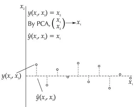
Fig.5 An example of unsupervised learning in system identification.

4.7 Gaussian process model

The reason why the curse of dimensionality occurs is due to the lack of a global model,so only local data can be used.The portion of the usable data gets smaller and smaller exponentially as the dimension of the problem gets higher and higher.Any global model even nonlinear would help in eliminating the curse of dimensionality problem.In this regard,Bayesian models,particularly Gaussian process model[19],is very useful.

In a Gaussian process model setting,let the noise be an independent Gaussian noise.Suppose that the unknown valuey0=f(x0)is what we are interested in.Assume thatf(x0),f(x(1)),...,f(x(N))follow a joint Gaussian distribution with zero mean(not necessary though)and a covariance matrix Σp.Lety0=f(x0),Y=(y(1) ···y(N))T.Since(y0,Y)Tfollows a jointGaussian,one has

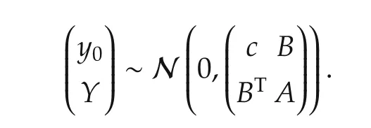
and the conditional mean is given by

The elegance is that every data can be used to establish the model and this avoids the curse of dimensionality problem.

4.8 Connection with regression

Variable selection is particularly important for the underling systems with the sparse representation.We start the problem with a linear case.

Let

where β∗=(β∗1···β∗p)Tand{εk,k=1,...,N}are iid random variables withEεk=0 andEε2klt; ∞.

The Lasso-type estimator is given by[20]

with λNvarying withN.

The adaptive Lasso estimator is given by[21]

Most of the existing results for Lasso and its variants are concerned with linear systems.Though the idea can be easily extended to a nonlinear case

its theoretical analysis is much involved.There are more and more results reported in the literature along this direction[22].

4.9 Parameter and set convergence

It is interesting to note from(3)in the previous section that variable selection involves not only parameter convergence but also set convergence.To illustrate,consider a case ofp=2 and

A∗is the set that determines which variable contributes and which one does not.Now let

This demonstrates that variable selection is more than parameter estimation.

5 Variable selection in nonlinear systems identif i cation

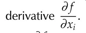
5.1 Top-down approach:two stages

wherehgt;0 is the bandwidth and O(h2)is the higher orderterms thatare ofnegligible orders whenx(k)−x0his close enough.

Let

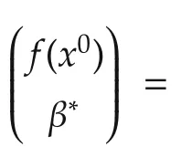
The local linear estimator(6)can be written as a least squares problem

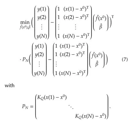
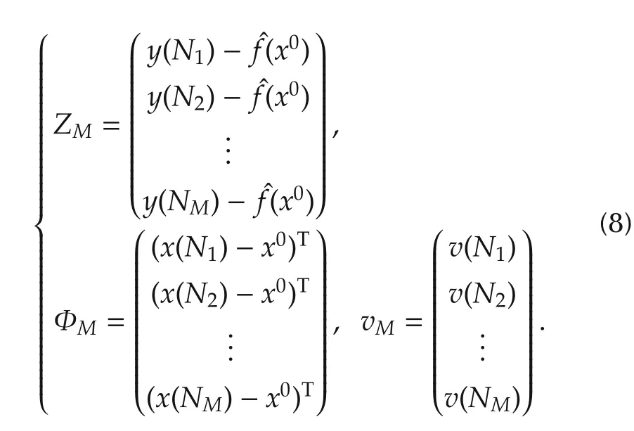
Ifx(k)is not in theh-neighborhood ofx0,thenKQ(x(k)−x0)=0.GivenN,h,letx(Ni)’s,i=1,...,Mbe in the neighborhood and lety(Ni)’s andv(Ni)’s be the corresponding output and noise sequences,respectively.Obviously,the numberM=M(N,h)of the regressors in the neighborhood depends on the total data lengthNand the bandwidthh.Letˆf(x0)be derived from the local linear estimator(6)or(7)and then define

By the standard results of the local linear estimator[24],we have

We now discuss the set convergence.For the variable selection problem,we assume that some variablesxi(k),1ipdo not contribute tof(·)in the neighborhood ofx0and so theIn other words,β∗is sparse or some elements of β∗=(β∗1···β∗p)Tare exactly zero.In particular,iffori∈[1,...,p],then we say that the variablexi(k)does not contribute.Without loss of generality,by re-arranging indices,we may assume that for some unknown 1qp,

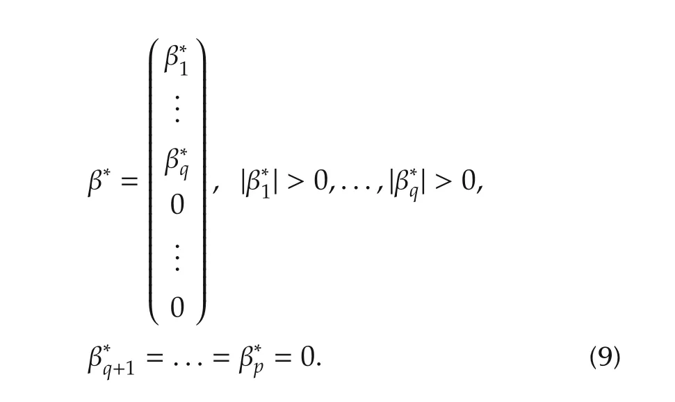
Define the true but unknown index set as

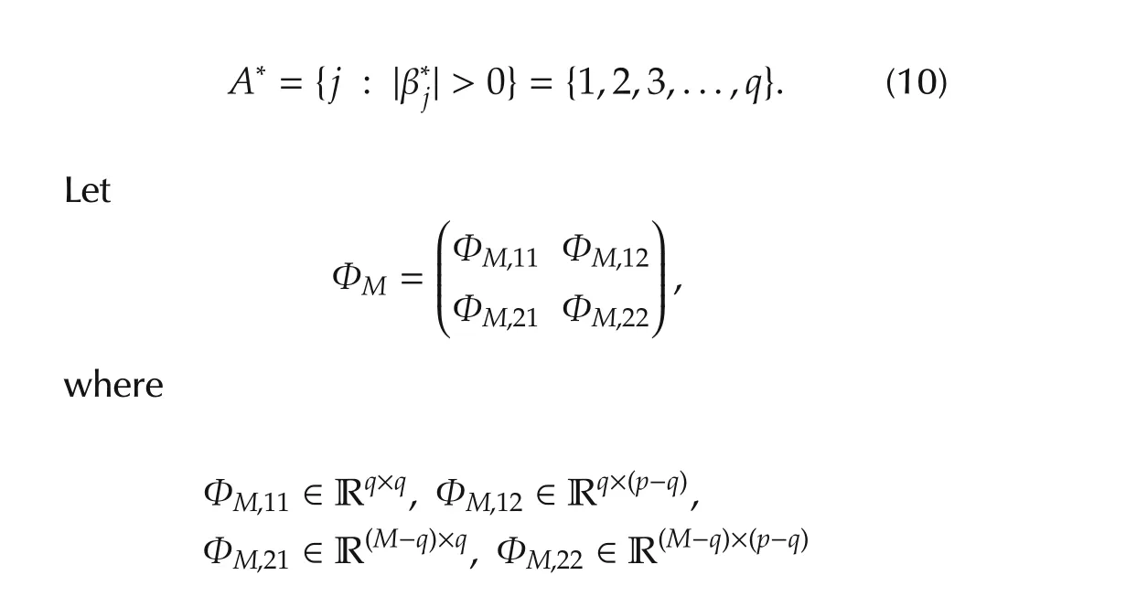
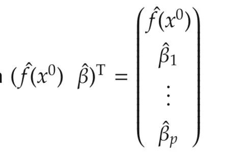
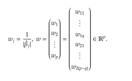
The approach is a convex penalized optimization,

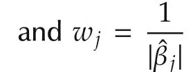
where β =(β1···βp)Tis the estimate derived from the penalized optimization(11).

Algorithm 1

Step2Collect all the regressors in thehneighborhood and the corresponding outputs.FormZMand ΦMas in(8).

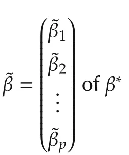
The goal is to establish the parameter and set convergence.The choice of λMandw jgiven above accomplishes this goal.We comment that other choices exist for the same goal.Interested readers are referred to[21]for further discussions.

To facilitate the convergence analysis,define

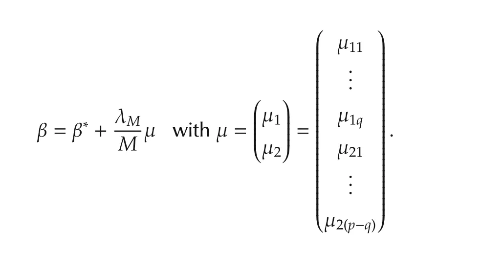
This variable change switches the problem of optimization with respect to β to a problem of optimization with respect to μ.The switch does not simplify the problem in terms of actual computation.It does however allow us to determine the conditions for the optimal μ2in terms of the true but unknown β∗in a much insightful way.Following the variable change,

Obviously,

SinceJ1(β∗)is a constant,we have

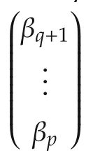
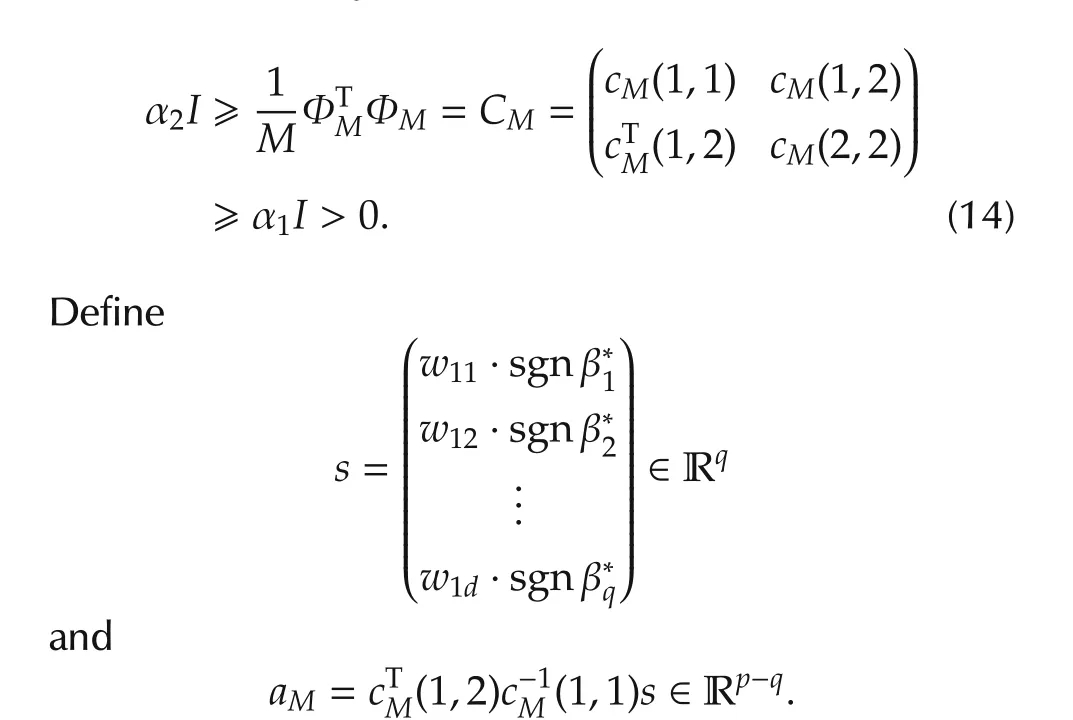
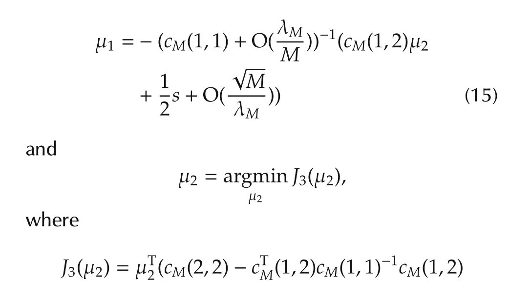
We remark thatthe condition(14)ofthe above lemma is a standard persistent excitation condition in the system identification literature.

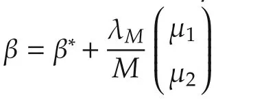
Lemma 2Under the conditions of Lemma 1,then for largeN,a sufficient condition for μ2=0 to be the minimizer ofJ3(μ2),i.e.,J3(μ2)gt;J3(0)for all μ2?0 is that

We now state the main result of the two stage approach.

Theorem 1Assume thatf(·)is twice differentiable atx0=(x01···x0p)T.Suppose thatxi(k)’s are iid with a continuous and positive density atx0i.Leth→0,Nhp+6→∞asN→∞.Then:

1)For eachNandh,letM(N,h)be the number of regressorsx(k)’s in theh-neighborhood ofx0and λM= γM2/3for some constant γ gt;0.Then,in probability asN→∞,

5.2 Top-down approach:Lasso-type algorithm

The algorithm presented in the previous section is a two stage algorithm.At the first stage the contributing variables are identified while at the second stage the parameters for the contributing variables are estimated.In fact,by appropriate modification on the algorithm the two stage procedure can be combined,i.e.,the consistent variable selection and parameter estimation can be achieved simultaneously.We present the results of[28]here.

Based on the definition for the local contributing variables given in the above section,the key steps towards variable selection of system(1)are to find a local linear model off(·)atx0and then to determine which coefficients in the local linear model are zero.Next,we first introduce an algorithm for identifying the local linear model off(·)atx0and then a penalized convex optimization algorithm for detecting the contributing variables.

with the kernel functionKk(x0)given by

Set

Then the estimates defined by(18)–(20)can be expressed by

In fact,θ0,Nand θ1,Nderived by the above algorithm serve as the estimates forf(x0)andf(x0),respectively.

Notice that the algorithm(22)is a standard form of weighted least squares estimator.Thus it can be easily formulated into a recursive version.

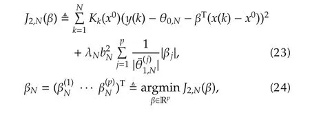
wherebkand the kernelKk(x0)are introduced in the local linear estimator,{λN}N1is a positive sequence tending to infinity and

forj=1,...,pand any fixed ε∈ (0,δ).

Similar to the above section,in the following we assume that there areq(p)contributing variables off(·)atx0,i.e.,there beingdnonzero elements in the gradient vectorf(x0).Set β∗f(x0).Without losing generality,we assume that β∗=(β∗1···β∗qβ∗q+1···β∗p)TandWhenever consistency of{θ1,N+1}N1takes place,we must have

Set since β∗(j)=0,j=q+1,...,p.Then,it is seen that

For the convergence analysis,we first introduce a set of conditions on the system.

A1)For the functionf(·)in the NARX system(1),it is with a second order derivative which is continuous atx0and|f(x)|c1xr+c2,∀x∈Rpfor some positive constantsc1,c2,andr.

A2){v(k)}k0is an iid sequence withEv(k)=0,0lt;Ev2(k)lt;∞;x(k)andv(k)are mutually independent for eachk1.

A3)The vector sequence{x(k)}k1is geometrically ergodic,i.e.,there exists an invariant probability measurePIV(·)on(Rp,B p)and some constantsc3gt;0 and 0lt; ρ1lt;1 such thatPk(·)−PIV(·)varc3ρk1,wherePk(·)is the marginal distribution ofx(k).PIV(·)is with a bounded pdf,denoted byfIV(·),which is with a continuous second order derivative atx0.

A4){x(k)}k1is an α-mixing with mixing coefficients{α(k)}k1satisfying α(k)c4ρk2for somec4gt;0 and 0lt;ρ2lt;1 andEx(k)rlt;∞fork1.

Conditions A3)and A4)are in fact on the asymptoticalstationarity and independence of{x(k)}k1.In general,conditions A3)and A4)hold true if the system satisfies some kinds of stability conditions and the input and the noise signals meet a certain of excitation requirements[29].

Next,we introduce the conditions on the algorithm.

A6)The sequence{λN}N1satisfies

where δgt;0 is given in A5).

Under the above assumptions,the strong consistency as well as the convergence rate of the local linear estimator can also be obtained.

Theorem2Assume thatA1)–A5)hold.Then itholds that

The following theorem establishes the strong consistency of the variable selection algorithm.

Theorem 3Assume that A1)–A6)hold.Then there exists an ω-set Ω0with P{Ω0}=1 such that for any ω∈Ω0,

i)there exists an integerN(ω)

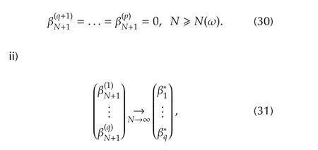
where{βN,N1}are generated from(24).

5.3 Bottom-up approach:global variable selection by stepsize algorithm

In this section,the global variable selection for system(1)is considered.Our focus is for a given pair ofn,p(nlt;p),to find thenmost important variablesxij(k),j=1,2,...,namongx1(k),x2(k),...,xp(k).Our idea is the minimum set of the unfalsified variables.To explain easily,let us say thatnvariables(xi1(k),xi2(k),...,xin(k))really contribute and the restp−nvariables do not.Then the set(xi1(k),...,xin(k))is the minimum set of the unfalsified variables,i.e.,for someg,

for allkindependent of the values ofx j(k)for allj?(i1,i2,...,in).Any set(x j(k),...,xˆn+j−1(k))for some ˆngt;nthat contains(xi1(k),xi2(k),...,xin(k))also has the property of unfalsified variables but is not the minimum set.On the other hand withˆnlt;n,there does not exist any functiongsuch that

for allk.

The algorithm starts at one variable[30],i.e.,to find the most important single variablexi(k)among allx1(k),x2(k),...,xp(k).To this end,a low dimensional neighborhood has to be defined.For each 1ipand eachx(k)=(x1(k),x2(k),...,xp(k)),k=1,2,...,N,we say thatx(j)is in the one dimensional neighborhoodhfor some smallhgt;0.Note thatx(k)isp-dimensional andxi(k)is one dimensional.The one dimensional neighborhood ofxi(k)is the collection ofx(j),j=1,2,...,Nformally defined by

wherecgt;0 is a scaling constant such that

Then the residual sum of squares(RSS)

could be used to determine whichxi(k)are the most important variable in terms of the smallest output error.We may say thatxi∗1(k)is the most important if

where RSSiis given by(35).

To find the second most important variable oncei∗1is obtained as defined in(36),choosei∈ (1,2,...,p)/i∗1,the correspondingxi(k)and define the neighborhood of(xi∗1(k),xi(k))similarly as in(33)by(37).

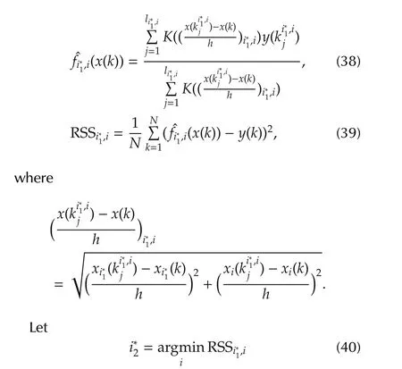
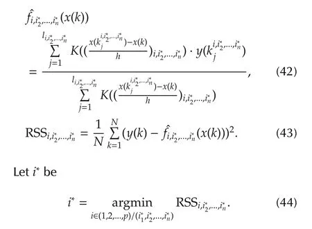
The idea of the algorithm is that RSS(43)monotonically decreases in the number of variables chosen when the number is less than the actual number of contributing variables.When the number of variables chosen is equal or larger than the actual number of contributing variables,RSS of(43)is flattened and does not decrease[31],as shown in the following theorem.

Theorem 4Consider system(1).Assume that A1)–A4)hold andh→0,hn N→∞asN→∞.Also assume that onlyn∗pvariables(1)and the chosen variable set(xi1(k),...,xin(k))con-Then for eachf(x(k))goes to zero asymptotically in probability asN→∞.

For illustration,we provide an example.In many applications,though variables are independent and not strictly on a low dimensional manifold,some only contribute marginally.The goal of variable selection is to find out which ones contribute insignificantly and then to remove these variables once identified for the identification purpose.This is different from the top-down approach.The example considered is given below,

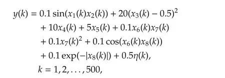
where 8 variables are independent and in fact iid random sequences uniformly in[−1,1],but the coefficients involvingx1,x2,x6,x7,x8are small so the contributions ofx1,x2,x6,x7,x8are insignificant compared to that ofx3,x4,x5.First,the residual sum of squares RSS vs the numbernof the variables chosen were calculated as shown in Fig.6 by the Forward/Backward selection algorithm which suggests that the dimensionn=3.Thus the Forward/Backward algorithm was applied by fixingn=3 to find 3 most dominate variables.In 100 Monte Carlo runs,the correct variablesx3,x4,x5were picked 100 times.Finally,to verify,a fresh validation datak=1,...,40 was generated in whichx1,x2,x6,x7,x8remained the same but Fig.7 shows the actualoutputand the estimated outputs by identifying the 8-dimensional system directly with GoF=0.5189 and by identifying a 3-dimensional systemy=g(x3,x4,x5)with GoF=0.9220.This example illustrates the usefulness of the bottom up approach.It is important to note that the data length is onlyN=500 for a 8-dimensional system.

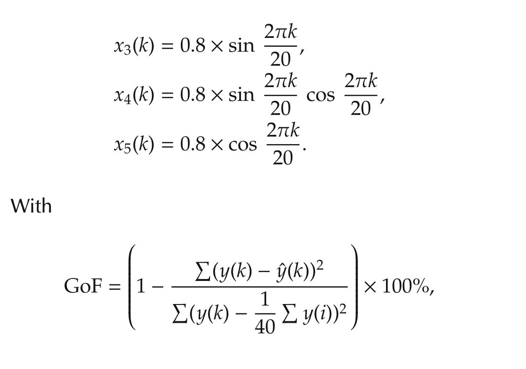
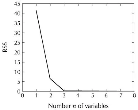
Fig.6 RSS vs the number n of variables.

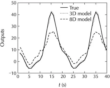
Fig.7 True output and the estimated outputs.

6 Conclusions

The problem of system identification for a high dimensional nonlinear non-parametric system has been examined from the variable selection perspective.It has been revealed that the formulated problem has strong connections to various problems in other research areas.Furthermore,some promising methods have been presented.This is a growing research area with great potentials.

[1]K.Li,J.Peng.Neuro input selection–a fast model based approach.Neurocomputing,2007,70(4/6):762–769.

[2] K.Li,J.Peng,E.W.Bai.A two-stage algorithm for identification of nonlinear dynamic systems.Automatica,2006,42(7):1189–1197.

[3] J.Peng,S.Ferguson,K.Rafferty,et al.An efficient feature selection method for mobile devices with application to activity recognition.Neurocomputing,2011,74(17):3543–3552.

[4] I.N.Lobato,J.Nankervis,N.Savin.Testing for zero autocorrelation in the presence of statistical dependence.Econometric Theory,2002,18(3):730–743.

[5]T.S¨oderstr¨om,P.Stoica.System Identification.New York:Prentice Hall,1989.

[6]C.Velasco,I.Lobato.A simple and general test for white noise.Proceedings of Econometric Society 2004 Latin American Meetings,Santiago,Chile,2004:112–113.

[7]S.Su,F.Yang.On the dynamical modeling with neural fuzzy networks.IEEE Transactions on Neural Network,2002,13(6):1548–1553.

[8]J.D.Bomerger,D.E.Seborg.Determination of model order for NARX models directly from input-output data.Journal of Process Control,1998,8(5/6):459–568.

[9]W.Zhao,H.-F.Chen,E.W.Bai,et al.Kernel-based local order estimation of nonlinear non-parametric systems.Automatica,2015,51(1):243–254.

[10]G.Pillonetto,M.Quang,A.Chiuso.A new kernel-based approach for nonlinear system identification.IEEE Transactions on Automatic Control,2011,56(12):2825–2840.

[11]X.Hong,R.T.Mitchell,S.Chen,etal.Modelselection approaches fornonlinearsystem identification:a review.InternationalJournal of Systems Science,2008,39(10):925–949.

[12]X.He,H.Asada.A new method for identifying orders of inputoutput models for nonlinear dynamic systems.Proceedings of the American Control Conference,San Francisco,CA:IEEE,2003:2520–2523.

[13]M.B.Kennel,M.R.Brown,H.Abarbanel.Determining embedding dimension for phase-space reconstruction using geometrical construction.Physical Review A,1992,45(6):3403–3411.

[14]L.Cao.Practical method for determining the minimum embedding dimension input-output models for nonlinear dynamic systems.Physica D:Nonlinear Phenomena,1997,110(1/2):43–50.

[15]S.Roweis,L.Saul.Nonlinear dimensionality reduction by local linear embedding.Science,2000,290(5500):2323–2326.

[16]D.Achlioptas.Database friendly random projections:Johnson-Lindenstrass with binary coins.Journal of Computer and System Sciences,2003,66(4):671–687.

[17]H.Ohlsson,J.Roll,T.Glad,et al.Using manifold learning for nonlinear system identification.Proceedings of the 7th IFACSymposium on Nonlinear Control Systems,Pretoria,South Africa:Elsevier,2007:170–175.

[18]J.Roll,A.Nazin,L.Ljung.Nonlinear system identification via direct weight optimization.Automatica,2005,41(3):475–490.[19]J.Kocijan,A.Girard,B.Banko,et al.Dynamic systems identification with Gaussian process.Mathematical and Computer Modelling of Dynamical Systems,2003,11(4):411–424.

[20]K.Knight,W.Fu.Asymptotics for Lasso-type estimators.The Annals of Statistics,2000,28(5):1356–1378.

[21]H.Zou.The adaptive Lasso and its oracle properties.Journal of American Statistical Association,2006,101(476):1418–1429.

[22]A.Arribas-Gil,K.Bertin,C.Meza,et al.LASSO-type estimators for semiparametric nonlinear mixed-effects model estimation.Statistics and Computing,2013,24(3):443–460.

[23]E.W.Bai,K.Li,W.Zhao,et al.Kernel based approaches to local nonlinear non-parametric variable selection.Automatica,2014,50(1):100–113.

[24]E.W.Bai.Non-parametric nonlinear system identification:an asymptotic minimum mean squared error estimator.IEEE Transactions on Automatic Control,2010,55(7):1615–1626.

[25]K.Mao,S.A.Billings.Variable selection in nonlinear system modeling.MechanicalSystems and SignalProcessing,2006,13(2):351–366.

[26]R.Mosci,L.Rosasco,M.Santoro,et al.Is there sparsity beyond additive models?Proceedings of the 16th IFAC Symposium on Systems Identification,Brussels,Belgium:Elsevier,2012:971–976.

[27]E.W.Bai,Y.Liu.Recursive direct weight optimization in nonlinear system identification:a minimal probability approach.IEEE Transactions on Automatic Control,2007,52(7):1218–1231.

[28]W.Zhao,H.-F.Chen,E.W.Bai,et al.Variable selection for NARX systems in first approximation.2015:http://user.engineering.uiowa.edu/erwei/VariableSelection.pdf.

[29]W.Zhao,W.Zheng,E.W.Bai.A recursive local linear estimator for identification of nonlinear ARX systems:asymptotical convergence and applications.IEEE Transactions on Automatic Control,2013,58(12):3054–3069.

[30]P.Peduzzi.A stepwise variable selection procedure for nonlinear regression methods.Biometrics,1980,36(3):510–516.

[31]G.E.P.Box,D.Pierce.Distribution of residual autocorrelations in autoregressive-integrated moving average time series models.Journal of American Statistical Association,1970,65(332):1509–1526.

Er-Wei BAIwas educated in Fudan University,Shanghai Jiaotong University,both in Shanghai,China,and the University of California at Berkeley.Dr.Bai is Professor and Chair of Electrical and Computer Engineering Department,and Professor of Radiology at the University of Iowa where he teaches and conducts research in identification,control,signal processing and their applications in engineering and life science.He holds the rank of World Class Research Chair Professor,Queen’s University,Belfast,U.K.Dr.Bai is an IEEE Fellow and a recipient of the President’s Award for Teaching Excellence and the Board of Regents Award for Faculty Excellence.E-mail:er-wei-bai@uiowa.edu.

Wenxiao ZHAOearned his B.Sc.degree from the DepartmentofMathematics,Shandong University,China in 2003 and a Ph.D.degree from the Institute of Systems Science,AMSS,the Chinese Academy of Sciences(CAS)in 2008.After this he was a postdoctoral student at the Department of Automation,Tsinghua University.During this period he visited the University ofWestern Sydney,Australia.Dr.Zhao then joined the Institute of Systems of Sciences,CAS in 2010.He now is with the Key Laboratory of Systems and Control,CAS as an Associate Professor.His research interests are in system identification,adaptive control,and system biology.He serves as the General Secretary of the IEEE Control Systems Beijing Chapter and an Associate Editor of the Journal of Systems Science and Mathematical Sciences.E-mail:wxzhao@amss.ac.cn.

†Corresponding author.

E-mail:er-wei-bai@uiowa.edu.Tel.:+1-319-335-5949;fax:+1-319-335-6028.

This work was partially supported by the National Science Foundation(No.CNS-1239509),the National Key Basic Research Program of China(973 program)(No.2014CB845301),the National Natural Science Foundation of China(Nos.61104052,61273193,61227902,61134013),and the Australian Research Council(No.DP120104986).

©2015 South China University of Technology,Academy of Mathematics and Systems Science,CAS,and Springer-Verlag Berlin Heidelberg

the B.Sc.degree in 1982,the M.Sc.degree in 1984,and the Ph.D.degree in 1989,all from Southeast University,Nanjing,China.He is currently a Professor at University of Western Sydney,Australia.Over the years he has also held various faculty/research/visiting positions at Southeast University,China;Imperial College of Science,Technology and Medicine,U.K.;University ofWestern Australia;Curtin University ofTechnology,Australia;Munich University of Technology,Germany;University of Virginia,U.S.A.;and University of California-Davis,U.S.A.Dr.Zheng is a Fellow of IEEE.E-mail:w.zheng@uws.edu.au.