Direct and noisy transitions in a model shear flow

Marina Pausch∗，Bruno Eckhardtb

aFachbereich Physik，Philipps-Universität Marburg，35032 Marburg，Germany

bJ.M.Burgerscentrum，Delft University of Technology，2628 CD Delft，The Netherlands

Direct and noisy transitions in a model shear flow

Marina Pauscha，∗，Bruno Eckhardta，b

aFachbereich Physik，Philipps-Universität Marburg，35032 Marburg，Germany

bJ.M.Burgerscentrum，Delft University of Technology，2628 CD Delft，The Netherlands

a r t i c l e i n f o

Article history：

Received 15 August 2014

Received in revised form

5 December 2014

Accepted 22 January 2015

Available online 23 April 2015

Transition to turbulence

Shear flows

Noise driven

Optimal initial conditions

The transition to turbulence in flows where the laminar profile is linearly stable requires perturbations of finite amplitude.‘‘Optimal’’perturbations are distinguished as extrema of certain functionals，and different functionals give different optima.We here discuss the phase space structure of a 2D simplified model of the transition to turbulence and discuss optimal perturbations with respect to three criteria: energy of the initial condition，energy dissipation of the initial condition，and amplitude of noise in a stochastic transition.We find that the states triggering the transition are different in the three cases，but show the same scaling with Reynolds number.

©2015 Published by Elsevier Ltd on behalf of The Chinese Society of Theoretical and Applied Mechanics. This is an open access article under the CC BY-NC-ND license（http://creativecommons.org/licenses/ by-nc-nd/4.0/）.

1.Introduction

In parallel shear flows like pipe flow，plane Couette flow or Poiseuille flow and in boundary layers like the asymptotic suction boundary layer or the Blasius profile，turbulence appears when the laminar profile is linearly stable against perturbations［1］.Accordingly，finite amplitude perturbations are required to trigger turbulence，a scenario referred to as by-pass transition［2］.Many studies in the above flows have shown that the transition to turbulence is associated with the presence of 3D exact coherent states［3］. They appear in saddle-node bifurcations which in the state space of the system create regions of initial conditions that do not decay to the laminar profile，but instead are attracted towards the nodestate［4］.As the Reynolds number increases，the region widens，the node state undergoes further bifurcations and chaotic attractors or saddles are formed［5-7］.Initial conditions can only trigger turbulence when they reach into thatinterior region，i.e.，cross the stable manifold of the saddle state on the boundary of the region［8］.An‘‘optimal’’perturbation is one that can trigger turbulence and at the same time is a minimum of a prescribed functional.Popular is an optimization based on amplification or energy gain over a given interval in time［9-17］or on the total time-averaged dissipation［18，19］.Because they take the time-evolution into account，they connect to optimization problems in control theory［20，21］.

We simplify matters here and focus on a geometric optimization by identifying initial conditions that will eventually become turbulent，without regard of the time it takes for them to become turbulent.The states are optimized so thata certain quadratic function，such as energy content or dissipation，is extremal:it is a maximum in the sense that all initial conditions with a lower value of the quadratic function will not become turbulent，and it is minimal in that the first initial conditions that become turbulent have values larger than this optimum.At the optimal value there will then be at least one trajectory which neither becomes turbulent nor returns to the laminar profile:it lies on the stable manifold of the edge state［8］，so that the optimum is reached when the isocontours of the optimization functional touch the stable manifold of the edge state（similar descriptions of the state space structure can be found in Refs.［17，19，22，23］）.

2.The Model

To fix ideas and to keep the mathematics as simple as possible，we take the 2D model introduced by Baggett and Trefethen［24］. The model we use is one of a set of many low-dimensional models of various levels of complexity［20，22，25-31］.It has a non-normal linear part and an energy conserving nonlinearity，and，this being the most important feature for the present application，it is 2D so that the entire phase space can be visualized（a property it shares with the illustrative model of Ref.［20］）.Despite its simplicity，the model can be used to illustrate several features of the transition mechanisms in shear flows.

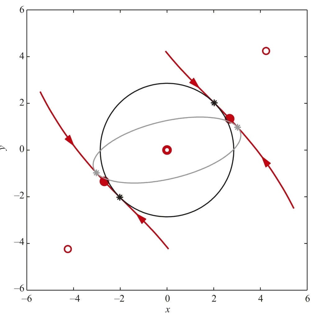
Fig.1.（Color online）State space of the 2D model for the transition to turbulence for R=3.The open symbols mark the stable fixed point at the origin（‘‘laminar’’state）and the two nodes from the bifurcation（‘‘turbulent’’states）.The full symbols are the edge states，and the red lines indicate the stable manifolds ofthe edge states. The black circle and the gray ellipsoid indicate the states where the energy（7）and the noise functional（12）are minimal，respectively.The points where they touch the stable manifolds are indicated by stars.

The model has two variables，which may be thought of as measuring the amplitudes of streaks x and vortices y（see also Ref.［32］），and one parameter R that plays the role of the Reynolds number

In order to highlight more clearly what happens near the origin，we magnify by rescaling the variables with the Reynolds number R（see Ref.［33］），i.e.，we redefine the amplitudes x=x′/R2，y=y′/R2and the time t=Rt′such that（with the primes dropped）

For R→ ∞，the saddles are to leading order in 1/R located at±（2，2/R），which in the original coordinates represents an approach to the origin like±（2/R2，2/R3）.The stable manifolds

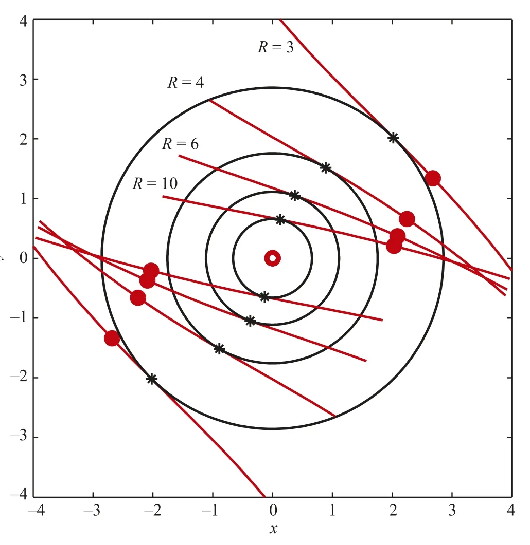
Fig.2.（Color online）Optimal states in energy for different R.The open symbol in the middle is the laminar state.States of fixed energy are indicated by circles，and the points where they touch the stable manifolds（red lines）of the edge states（indicated as full symbols）are the points marked by stars.One notes that as R increases，the manifolds become more parallelto the x-axis，and the pointofcontact approaches the origin from the y-axis.

rotate so as to become parallel to the x-axis，as we will see in the following.

3.Optimal Initial Conditions of Minimal Energy

The Euclidean distance to the origin can be obtained from a quadratic form

which has the form of kinetic energy.This assignment is further supported by the observation that E is preserved under time evolution by the nonlinear terms alone.In the sense described in the introduction，optimality with respect to this energy functional thus means the largest value up to which all trajectories return to the laminar state，and the smallest one where the first trajectories that evolve towards the turbulent state become possible.On the boundary between these two cases are states that neither return to laminar nor become turbulent，that lie on the stable manifold of the edge state.Geometrically，we are thus looking for the circle with the largest radius that we can draw around the origin that justtouches the stable manifold.Algorithmically，we find this point by a modified edge tracking which minimizes the energy（7）as described in the Appendix.

An example of such an optimal circle is given in Fig.1，and its variation with R is shown in Fig.2.As the Reynolds number increases，the fixed point moves towards（2，0）on the abscissa，and the stable manifold rotates to being parallel to the abscissa. The point of contact between circles of equal energy and the stable manifold moves away from the edge state，approaches the y-axis and moves inwards to the origin like 1/R.

In an insightful discussion of the energy functional，Cossu［23］notes that in the time-derivative of the energy functional only the linear parts of the equations of motion remain and that the nonlinear ones drop out because energy is preserved.This observation allows to define a necessary condition for the location

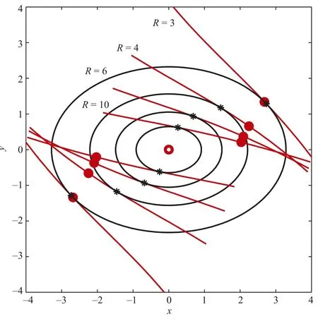
Fig.3.（Color online）Optimal states with respect to the dissipation functional for different R.States offixed dissipation are indicated by ellipses，and the points where they touch the stable manifolds（red lines）of the edge states（full symbols）are marked by stars.The open symbol in the middle is the laminar state.One notes that as R increases，the point of contact moves very much as in the case of the energy functional.

of the extremum，which for the 2D example studied here implies thatthe optimumlies along the line connecting the laminarand the turbulent fixed points.One could then find the optimum by a onedimensional search along this line.However，we did not pursue this further，as we also want to find optima with respect to other functionals that are not preserved by the nonlinear terms.

4.Optimal Initial Conditions of Minimal Energy Dissipation

The diagonal terms in the linear part of the equations of motion correspond to the dissipation in the original Navier-Stokes equation.Accordingly，we can define a dissipation functional［18］ϵ=（1/2）（x2+2y2） （8）and study initial conditions that are minimal or optimal with respect to this functional.As in the previous example，the geometrical condition is that we now have to find the point where an ellipse touches the stable manifolds.This gives the ellipses shown for different R in Fig.3.Note that the points where the ellipses touch the stable manifolds are different from the ones of the energy functional，but their asymptotic behavior for large R seems to be similar（see below）.

5.Optimal Noisy Transitions

As a third example we consider noise-driven transitions.To this end，the equations of motion are expanded to include a stochastic forcing of the individual terms，

where the noise is characterized by〈ξi〉=0 and〈ξi（t）ξj（t′）〉= Dijδi，j.We consider the case D11=D22=D，so that both components are driven with equal noise amplitude.In a linear approximation around the laminar fixed point，the non-normal coupling

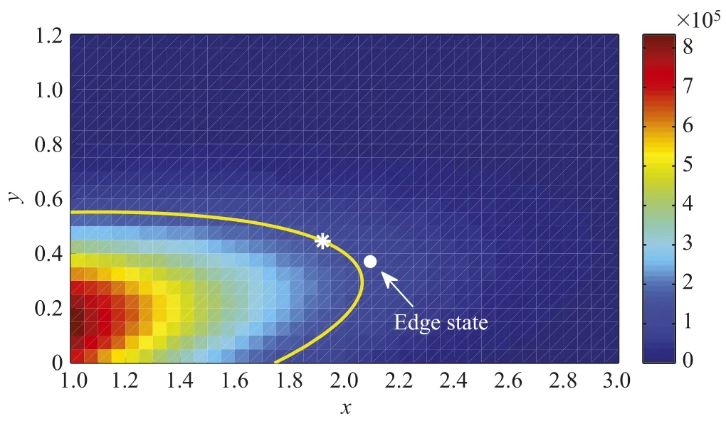
Fig.4.Probability density for the linearized equations with noise for R=6 in the region of phase space where the transition is expected to occur.For the statistics we calculated the time evolution of 20000 initial conditions starting at the laminar state for 20 time units with a step size of d t=10−3.It can be seen that the isocontours p=const.are of elliptical shape.The star indicates the point where the noise functional touches the stable manifold of the edge state.

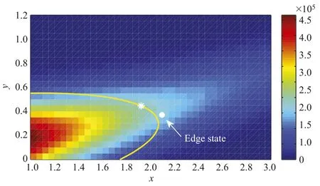
Fig.5.Probability density as in Fig.4，but for the full nonlinear equations with noise.Note that the iso-contours of equal probability are stretched out towards the turbulent state and that they cross the stable manifold close to the point of contact indicated as the optimal state.

between the two components results in a probability density function（pdf）for the two components that is Gaussian with a covariance matrix［34］given by

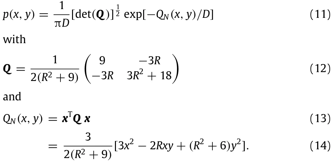
Asymptotically，for R→∞，the quadratic form becomes QN（x，y）→3y2/2，so that the Gaussian stretches out along the x-direction for increasing R.

In the noisy case，transition is induced when a fluctuation carries the system across the stable manifold.A good estimate of the likelihood of transition can be obtained by considering the probability density at the transition point.Given the functional form of the pdf，the biggest contribution to its variations comes from the quadratic form in the exponent.The equation shows that the iso-contours p = const.are ellipsoids determined by QN=const.that decrease or increase with the noise amplitude D.Therefore，if we want to describe where a noisy trajectorycrosses over to the turbulent state，we again have to study isocontours of a quadratic form，QN=const.，and determine where they touch the stable manifold of the saddle state.In contrast to the energy functional（7）and the dissipation functional（8），the fluctuation functional QNdepends on the Reynolds number. The point of contact between the probability iso-contours and the stable manifold then corresponds to the point where trajectories are most likely to cross over the stable manifold and to become turbulent.Alternatively，ifone wants to push the system to become turbulent，small perturbations in that region are most effective because the border is so close.

Figures 4 and 5 show the relative probability density to be at（x，y）in the region where the transition is expected to occur.It is obtained by integrating 20000 initial conditions in time for 20 time units starting at the laminar state with a step size of d t= 10−3.As the phase space is symmetric with respect to the origin，trajectories from the third quadrant are mirrored into the first quadrant.Figure 4，obtained without the nonlinear part，shows the Gaussian shape ofthe iso-contours.Outofthe 400×106calculated points of the trajectories，more than 108×106lay in the plotted region of phase space.In Fig.5 the nonlinear part is added and the pdf stretches out along the path to the turbulent state.The figure shows clearly that this happens close to the point where the ellipsoid QN（x，y）=const.touches the stable manifold.Here more than 75×106points lay in the interesting region ofphase space.We note that the shape of the iso-contours of the pdf is independent of the noise amplitude D（within the linear approximation），so that changes in D will predominantly influence the likelihood of a transition，but not the path it takes.

More examples of such iso-contours are shown in Figs.1 and 6 for different values of R.With increasing R the ellipsoids become more elongated in x-direction，as a resultofthe asymptotic behavior of the quadratic form noticed above（14）.As they are rotated in the direction opposite to the rotation of the stable manifolds，the point of contact stays close to the edge state.Within the hydrodynamic interpretation，the transition is dominated by the streaks（x-component）that form as a result of the vortices（ycomponent），not by the vortices themselves.

6.Summary and Conclusions

The calculations illustrate how different optimization criteria select different optimal initial conditions for the transition to turbulence.Geometrically，this is to be expected since different quadratic forms give rise to different ellipsoids in their isocontours and hence also different points of contact with the stable manifolds.We note that the results of Ref.［13］suggest that for optimization with a time-integrated functional the difference between energy and dissipation functionals is smaller and may actually vanish.However，we have not pursued this question further.

The variation of the optimal points of contact is summarized in Fig.7.The data indicates that while the optimal perturbations are vortex like for the energy and the dissipation functional，they are streak like for the noisy transition.The difference can be rationalized by the different dynamics.In the deterministic cases，with the energy and the dissipation functional，small vortex like initial conditions can grow in time to develop the streaks which then drive the transition.The noisy system is always exposed to small perturbations which can grow to develop streaks，so that the pdf is elongated in the streak direction by non-normal amplification.Therefore，the transition happens on top of the already existing streaks and noise driven flows［35-37］may show different structures at the point of transition than flows driven by judiciously chosen initial conditions.

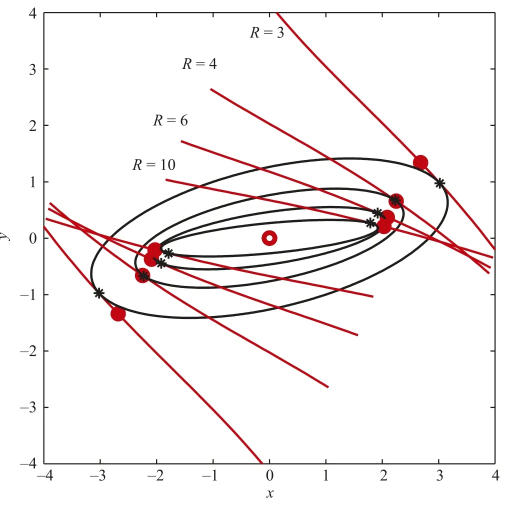
Fig.6.（Color online）Isocontours of the probability density function for different R.Note that as R increases，the ellipsoids of the iso-contour become narrower in the y-direction and stretch out along the x-direction.In combination with the rotation of the stable manifolds（red lines）the point of contact（stars）now stays close to the edge state（full symbols）and moves towards the x-axis.This is physically plausible，as a small perturbation in y（in the vortex direction）will produce a strong streak in the x-direction，and it is then the streak that triggers the transition.

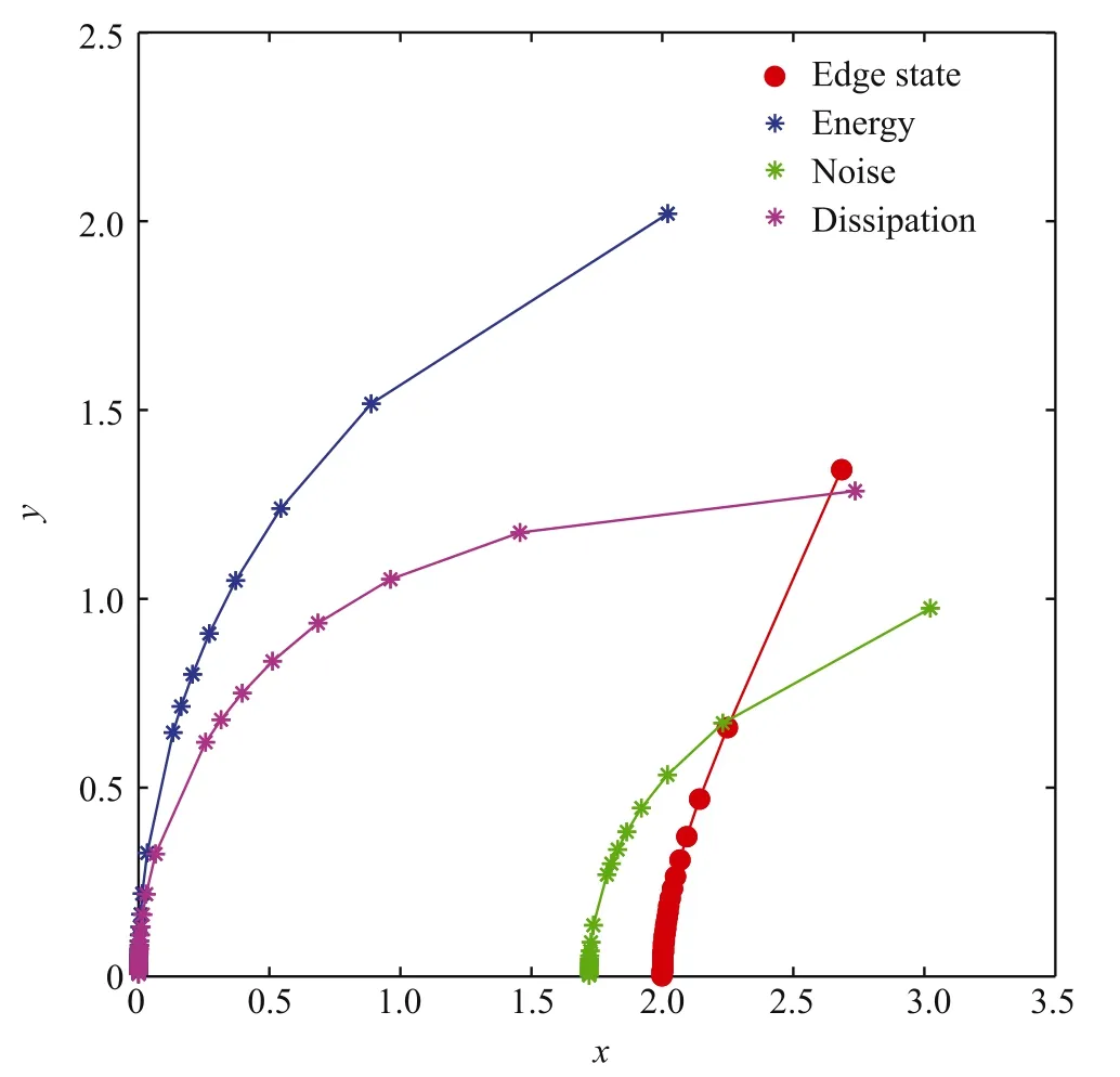
Fig.7.（Color online）Location ofthe points ofcontact.The top graph shows that for the energy and dissipation functional the optimal perturbations are vortex like and move towards the origin along the y-axis.The noise-optimals are more streak-like and move towards the x-axis，and actually remain close to the edge state.The edge state（red bullets）approaches（2，0）with R→∞.

A final quantity to study is the scaling of the functional with Reynolds number，as shown in Fig.8.Despite the differences in dynamics，the functionals scale in all three cases like 1/R2for large R. The particular exponent is specific to the model studied here and the type and formofthe nonlinearinteractions，as othernonlinearities can require a rescaling near the origin［38］.However，the fact that all three cases show the same scaling could also apply to the full flow cases，as it is a consequence of the measure used and notthe particular nonlinearity at play.What the model also shows is that deviations from the asymptotic behavior appear close to the point of bifurcation.It is tempting to speculate that such effects may be responsible for the different critical exponents that have been observed in pipe flow or plane Couette flow，but that clearly requires the transfer of the present analysis to realistic flow simulations and a careful analysis of the asymptotic properties.

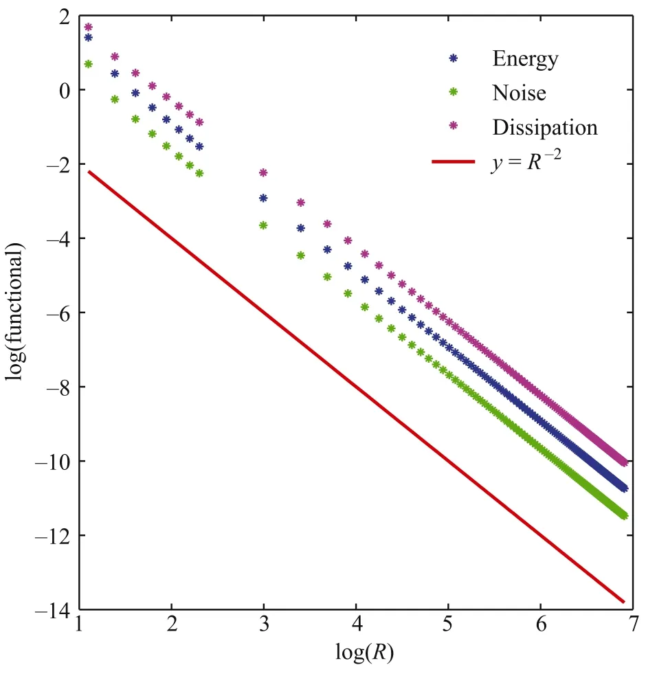
Fig.8.Scaling of the functionals for the optimal perturbations.Even though the point of contact moves differently，the critical values decay like 1/R2in all three cases.

The analysis of simple models has repeatedly helped to elucidate many features of the transition to turbulence in shear flows，and to develop tools to explore them ［20，22，25-31］.It is in this spirit that we have used a forward integration technique to find the optimal points on the stable manifolds for different functionals and to explore the changes with Reynolds number. We expect that many of the features described here can also be found in the high-dimensional state spaces of realistic shear flows，perhaps after suitable modifications and adaptations of the methods used to explore the high-dimensional spaces.

Acknowledgments

This work was supported in part by the German Research Foundation within FOR 1182.

Appendix

In this appendix we discuss the modification of the edge tracking algorithm ［8］used for the determination of the initial conditions on the edge that optimize a prescribed quadratic functional QN（x，y）.The functional may be the energy（7），the dissipation（8）orthe argumentin the pdf（12）.To keep the notation compact，we denote the equations of motion in vectorial notation as˙x=f.

We begin with an arbitrary initialcondition in the vicinity ofthe edge and we let it evolve in time towards the edge state.Unlike other edge tracking methods，where trajectories are integrated until they are sufficiently close to the laminar or the turbulent state，we here stop the integration at the time when the distance to the edge state is minimal.The trajectory’s velocity at the turning pointis then projected onto the normalofthe stable eigenvector to decide ifthe tested initialcondition moves upwards ordownwards，towards the turbulent or the laminar state.With this criterion we can determine a point x0on the edge also when the point is very close to the edge and the time needed to pass the edge state becomes excessively large.

We then propagate this point along the time direction，x1= x0+s f（x0）by an amount s that is chosen such that Q（s）is minimized.Formally，

In numerical implementations，∥s f∥is kept below a certain threshold to stay in a region where linear approximations are possible.Then a new edge tracking is started from x1and the process is repeated untilthe norm ofthe totalshift∥s f∥falls below a convergence threshold，here 10−5.

［1］S.Grossmann，The onset ofshear flow turbulence，Rev.Modern Phys.72（2000）603-618.http://dx.doi.org/10.1103/RevModPhys.72.603. http://adsabs. harvard.edu/cgi-bin/nph-data_query？bibcode=2000RvMP...72..603G&link_ type=ABSTRACT.

［2］M.V.Morkovin，Critical evaluation of transition from laminar to turbulent shear layers with emphasis on hypersonically traveling bodies.DTIC Document，1969.http://oai.dtic.mil/oai/oai？verb=getRecord& metadataPrefix=html&identifier=AD0686178.

［3］B.Eckhardt，Turbulence transition in pipe flow:some open questions，Nonlinearity 21 （2007） T1-T11.http://dx.doi.org/10.1088/0951-7715/ 21/1/T01. http://stacks.iop.org/0951-7715/21/i=1/a=T01？key=crossref. d91cf9a0cfb29103f99ef13e660a4248.

［4］T.Kreilos，B.Eckhardt，Periodic orbits near onset of chaos in plane Couette flow，Chaos 22（2012）047505.http://dx.doi.org/10.1063/1.4757227. http://link.aip.org/link/CHAOEH/v22/i4/p047505/s1&Agg=doi.

［5］F.Mellibovsky，B.Eckhardt，Takens-Bogdanov bifurcation of travelling-wave solutions in pipe flow，J.Fluid Mech.670（2011）96-129.http://dx.doi.org/ 10.1017/S0022112010005239.http://www.journals.cambridge.org/abstract_ S0022112010005239.

［6］F.Mellibovsky，B.Eckhardt，From travelling waves to mild chaos:a supercritical bifurcation cascade in pipe flow，J.Fluid Mech.709（2012）149-190.http://dx.doi.org/10.1017/jfm.2012.326. http://www.journals.cambridge.org/abstract_S0022112012003266.

［7］J.Halcrow，J.F.Gibson，P.Cvitanović，D.Viswanath，Heteroclinic connections in plane Couette flow，J.Fluid Mech.621（2009）365-376.http://dx.doi.org/ 10.1017/S0022112008005065.http://www.journals.cambridge.org/abstract_ S0022112008005065.

［8］J.D.Skufca，J.A.Yorke，B.Eckhardt，Edge of chaos in a parallel shear flow，Phys.Rev.Lett.96（2006）174101.http://dx.doi.org/10.1103/PhysRevLett.96. 174101.http://link.aps.org/doi/10.1103/PhysRevLett.96.174101.

［9］D.Biau，A.Bottaro，An optimal path to transition in a duct，Phil.Trans.R.Soc.A 367（1888）（2009）529-544.http://dx.doi.org/10.1126/science.261.5121.578. http://rsta.royalsocietypublishing.org/cgi/doi/10.1098/rsta.2008.0191.

［10］C.C.T.Pringle，R.R.Kerswell，Using nonlinear transient growth to construct the minimal seed for shear flow turbulence，Phys.Rev.Lett. 105 （2010） 154502.http://dx.doi.org/10.1103/PhysRevLett.105.154502. http://link.aps.org/doi/10.1103/PhysRevLett.105.154502.

［11］C.C.T.Pringle，A.P.Willis，R.R.Kerswell，Minimal seeds for shear flow turbulence:using nonlinear transient growth to touch the edge of chaos，J.Fluid Mech.702（2012）415-443.http://dx.doi.org/10.1017/jfm.2012.192. http://www.journals.cambridge.org/abstract_S0022112012001929.

［12］S.M.E.Rabin，C.P.Caulfield，R.R.Kerswell，Variational identification of minimal seeds to trigger transition in plane Couette flow，2011. http://arxiv.org/abs/1111.6654.

［13］S.M.E.Rabin，C.P.Caulfield，R.R.Kerswell，Triggering turbulence efficiently in plane Couette flow，J.Fluid Mech.712（2012）244-272.http://dx. doi.org/10.1017/jfm.2012.417.http://www.journals.cambridge.org/abstract_ S002211201200417X.

［14］S.Cherubini，J.C.Robinet，A.Bottaro，P.De Palma，Optimal wave packets in a boundary layer and initial phases of a turbulent spot，J.Fluid Mech.656（2010）231-259.http://dx.doi.org/10.1017/S002211201000114X. http://www.journals.cambridge.org/abstract_S002211201000114X.

［15］S.Cherubini，P.De Palma，J.C.Robinet，A.Bottaro，Rapid path to transition via nonlinear localized optimal perturbations in a boundary-layer flow，Phys. Rev.E 82（2010）066302.http://dx.doi.org/10.1103/PhysRevE.82.066302. http://link.aps.org/doi/10.1103/PhysRevE.82.066302.

［16］S.Cherubini，P.De Palma，Nonlinear optimal perturbations in a Couette flow:bursting and transition，J.Fluid Mech.716（2013）251-279. http://dx.doi.org/10.1017/jfm.2012.544. http://adsabs.harvard.edu/cgibin/nph-data_query？bibcode=2013JFM...716..251C&link_type=EJOURNAL.

［17］S.Cherubini，P.De Palma，Minimal perturbations approaching the edge of chaos in a Couette flow，Fluid Dyn.Res.46（2014）http://dx.doi.org/10.1088/ 0169-5983/46/4/041403.http://stacks.iop.org/1873-7005/46/i=4/a=041403.

［18］A.Monokrousos，A.Bottaro，L.Brandt，A.Di Vita，D.S.Henningson，Nonequilibrium thermodynamics and the optimal path to turbulence in shear flows，Phys.Rev.Lett.106（2011）134502.http://dx.doi.org/10.1103/PhysRevLett. 106.134502.http://link.aps.org/doi/10.1103/PhysRevLett.106.134502.

［19］Y.Duguet，A.Monokrousos，L.Brandt，D.S.Henningson，Minimal transition thresholds in plane couette flow，Phys.Fluids 25（2013）084103.http://dx.doi. org/10.1063/1.4817328.http://scitation.aip.org/content/aip/journal/pof2/25/ 8/10.1063/1.4817328.

［20］R.R.Kerswell，C.C.T.Pringle，A.P.Willis，An optimisation approach for analysing nonlinear stability with transition to turbulence in fluids as an exemplar，Rep. Progr.Phys.77（2014）http://dx.doi.org/10.1088/0034-4885/77/8/085901. http://stacks.iop.org/0034-4885/77/i=8/a=085901.

［21］P.Luchini，A.Bottaro，Adjoint equations in stability analysis，Annu.Rev. Fluid Mech.46（2014）493-517.http://dx.doi.org/10.1146/annurev-fluid-010313-141253.http://www.annualreviews.org/doi/abs/10.1146/annurevfluid-010313-141253.

［22］O.Dauchot，P.Manneville，Local v ersus global concepts in hydrodynamic stability theory，J.Phys.II France 7（1997）371-389.http://dx.doi.org/10.1051/ jp2:1997131.http://dx.doi.org/10.1051/jp2:1997131.

［23］C.Cossu，An optimality condition on the minimum energy threshold in subcritical instabilities，C.R.Mécanique 333（2005）331-336.http://dx. doi.org/10.1016/j.crme.2005.02.002.http://www.sciencedirect.com/science/ article/pii/S1631072105000379.

［24］J.S.Baggett，L.N.Trefethen，Low-dimensional models of subcritical transition to turbulence，Phys.Fluids 9（1997）1043-1053.http://dx.doi.org/ 10.1063/1.869199. http://adsabs.harvard.edu/cgi-bin/nph-data_query？bibcode=1997PhFl....9.1043B&link_type=EJOURNAL.

［25］T.Gebhardt，S.Grossmann，Chaos transition despite linear stability，Phys. Rev.E 50（1994）3705-3711.http://dx.doi.org/10.1103/PhysRevE.50.3705. http://adsabs.harvard.edu/cgi-bin/nph-data_query？bibcode=1994PhRvE..50. 3705G&link_type=ABSTRACT.

［26］F.Waleffe，Transition in shear flows.Nonlinear normality versus nonnormal linearity，Phys.Fluids 7 （1995）3060-3066.http://dx.doi.org/ 10.1063/1.868682. http://adsabs.harvard.edu/cgi-bin/nph-data_query？bibcode=1995PhFl....7.3060W&link_type=EJOURNAL.

［27］B.Eckhardt，A.Mersmann，Transition to turbulence in a shear flow，Phys.Rev. E 60（1999）509-517.http://dx.doi.org/10.1103/PhysRevE.60.509.http:// adsabs.harvard.edu/cgi-bin/nph-data_query？bibcode=1999PhRvE..60..509E& link_type=ABSTRACT.

［28］J.Moehlis，H.Faisst，B.Eckhardt，A low-dimensional model for turbulent shear flows，New J.Phys.6（2004）56-56.，http://stacks.iop.org/1367-2630/6/i=1/ a=056？key=crossref.9a9df4ab9f646cd3ca0a9aacaaaa7597.

［29］J.Moehlis，H.Faisst，B.Eckhardt，Periodic orbits and chaotic sets in a low-dimensional model for shear flows，SIAM J.Appl.Dyn.Syst.4（2005）352-376.http://dx.doi.org/10.1137/040606144.http://epubs.siam.org/doi/ abs/10.1137/040606144.

［30］N.R.Lebovitz，Shear-flow transition:the basin boundary，Nonlinearity 22（2009）2645-2655.http://dx.doi.org/10.1088/0951-7715/22/11/004. http://stacks.iop.org/0951-7715/22/i=11/a=004？key=crossref. 0e58a5bcc8174f507f138b3f9267a33c.

［31］N.Lebovitz，G.Mariotti，Edges in models of shear flow，J.Fluid Mech.721（2013）386-402.http://dx.doi.org/10.1017/jfm.2013.38. http://adsabs. harvard.edu/cgi-bin/nph-data_query？bibcode=2013JFM...721..386L&link_ type=EJOURNAL.

［32］B.Eckhardt，R.Pandit，Noise correlations in shear flows，Eur.Phys.J. B 33 （2003） 373-378. http://dx.doi.org/10.1140/epjb/e2003-00178-3. http://www.springerlink.com/Index/10.1140/epjb/e2003-00178-3.

［33］B.Eckhardt，K.Marzinzik，A.Schmiegel，Transition to turbulence in shear flows，in:A Perspective Look at Nonlinear Media，Springer，1998，pp.327-338.http: //dx.doi.org/10.1007/BFb0104973.http://link.springer.com/chapter/10.1007/ BFb0104973.

［34］H.Risken，The Fokker-Planck Equation，third ed.，in:Springer Series in Synergetics，Springer，1996.

［35］J.V.Sengers，J.M.Ortiz de Zárate，Velocity fluctuations in laminar fluid flow，J.Non-Newton.Fluid Mech.165（2010）925-931.http://dx.doi.org/ 10.1016/j.jnnfm.2010.01.020. http://linkinghub.elsevier.com/retrieve/pii/ S0377025710000224.

［36］J.M.Ortiz de Zárate，J.V.Sengers，Hydrodynamic fluctuations in laminar fluid flow.I.Fluctuating Orr-Sommerfeld equation，J.Stat.Phys.144（2011）774-792.http://dx.doi.org/10.1007/s10955-011-0256-1. http://link.springer.com/10.1007/s10955-011-0256-1.

［37］J.M.Ortiz de Zárate，J.V.Sengers，Hydrodynamic fluctuations in laminar fluid flow.II.Fluctuating squire equation，J.Stat.Phys.150（2012）540-558. http://dx.doi.org/10.1007/s10955-012-0495-9. http://link.springer.com/10.1007/s10955-012-0495-9.

［38］B.Eckhardt，D.P.Lathrop，Nonlinear normal forms for non-normal fixed points，Nonlinear Phenom.Complex Syst.9（2006）133-140.http://www.jnpcs.org/abstracts/vol2006/v9no2/v9no2p133.html.

∗Corresponding author.

E-mail address：marina.pausch@physik.uni-marburg.de（M.Pausch）.

http://dx.doi.org/10.1016/j.taml.2015.04.003

2095-0349/©2015 Published by Elsevier Ltd on behalf of The Chinese Society of Theoretical and Applied Mechanics.This is an open access article under the CC BY-NC-ND license（http://creativecommons.org/licenses/by-nc-nd/4.0/）.

*This article belongs to the Fluid Mechanics