Developing a Computer Program for Detailed Study of Planing Hull’s Spray Based on Morabito’s Approach

Parviz Ghadimi, Sasan Tavakoli, Abbas Dashtimanesh and Arya Pirooz

1. Department of Marine Technology, Amirkabir University of Technology, Tehran 15875-4413, Iran

2. Faculty of Engineering, Persian Gulf University, Bushehr 7516913817, Iran

3. International Branch, Amirkabir University of Technology, Tehran 15875-4413, Iran

1 Introduction1

The motion of a planing hull leads to evolution of two patterns of water spray each of which is comprised of a distinct geometry. Geometry of these patterns have been displayed by Savitsky and Breslin (1958). In the longitudinal and top views of the planing hull, there is a pattern which looks like a flat sheet. This pattern is called “whisker spray”.There is also another spray pattern that bears resemblance to a cone which is known as the “main spray”. The existence of the main spray leads to the definition of a parameter called“spray apex”. This parameter represents a point with highest vertical position of the main spray.

In the early 1930s, water spray of planing hulls was investigated on a preliminary level. At early stages, these studies included water sprays in planing plates. Wagner (1932)undertook the first study of the spray of infinite and semi-infinite planing flat plates. Subsequently, Sottorf (1932)experimentally studied sprays in planing hulls. As a result, he stated that the main reason for spray generation in planing hulls is variation of pressure from maximum values on the stagnation line to zero at the spray root. On the other hand,Lock (1943) studied geometry of the spray apex through experimental methods. Later, Green (1935, 1936) conducted one of the most significant studies in this field. He considered a planing flat plate of finite length and developed an analytical method to obtain appropriate equations for the lift, spray thickness, and other characteristics of planing motion.However, the most essential result of his studies, which is utilized in the current study, is related to the position of the stagnation point. He showed that if the distance from the stagnation point to the trailing edge starts to decline, then there will be some alterations in spray characteristics including rotation of spray to the aft of the plate and an increase in the spray thickness.

Pierson and Leshnover (1950) separated the bottom area of the planing hull into pressure and spray areas. They found that stagnation line is one of the essential factors which have important effect on the water spray. Their studies became the initial point of Savitsky and Breslin’s (1958) proposal of planes being normal to stagnation line. As a result, they were able to explain the process of spray formation by means of the phenomena discussed by Green (1936). Based on the idea presented by Savitsky and Breslin (1958), analytical solutions by Green (1936) can be used in any section normal to the stagnation line. The spray can subsequently be modeled by considering each section as a planing plate in which position of the stagnation point is different with respect to the other. As discussed previously, in Green’s approach (1936), it was shown that as the stagnation point converges towards the trailing edge, the spray rotates to the aft of the plate. As a result, it is evident that in the last sections where the stagnation line crosses the chine, there will be a rotation of the spray. This rotation is the cause of main spray in planing hulls.Generation of the whisker spray can be explained by the analysis of the sections in which the stagnation point is far from the leading edge and there would not be any radical changes in the spray flow. This fact proves that spray flows towards the left side of these sections, with an angle between the plate and the water. By intensifying the result of these sections, a flat sheet of water will be produced.

When the computational method for modeling the steady planing in calm water was introduced by Savitsky (1964),there was a change in the means of studying planing vessels.For instance, Zarnick (1978) tried to develop different models for predicting steady planing and additional motions of these crafts in rough water. An important study was also done by Kikuhara (1960) based on experimental modeling of spray formation using the 2D+ttheory. He drew on the results of water entry in wedge section bodies for the study of water spray. His results were the main motivation behind the numerical study done by Kihara (2006).

Determining characteristics of free surface in water entry problems is one of the key techniques in predicting spray in planing crafts. Different authors have used numerical,analytical and experimental methods to accomplish this task.In an important work, Payne (1986, 1989) used added mass theory to investigate water spray at constant velocity water impact. First, spray on a flat plate and then spray on water entry of a wedge were evaluated. He also obtained the trajectory of spray in planing vessels using his analytical method. Lattore and Ryan (1989) tried to further develop Savisky and Breslin’s (1958) idea of using projectile theory in dynamics. Savitskyet al. (2007) presented a new method for calculating the resistance of whisker spray. Determination of reflection of flow by stagnation line was the result of their study.

The focal point of all the previous studies about spray is summarized in the study completed by Morabito (2010). He presented several new equations for prediction of the spray.His method was based on the proposal presented by Savitsky and Breslin (1958). Combination of several equations associated with the normal sections about the stagnation line and geometry of the craft were the most essential aspect of his work. Subsequently, Savitsky and Morabito (2011) presented various new experimental results regarding spray and derived an equation for calculating the location of spray in planing hulls. This venture, which was based on swept wing theory, is indeed the basic scheme which made use of planes normal to the stagnation line. In this theory, two components are considered for the velocity vector; normal to the stagnation line and along the stagnation line. Using the proposed equations by Morabito (2010), the modeling of water spray becomes possible by considering a particular computational process which is introduced in the current study.

In this paper, a computational process is systematically developed to facilitate the prediction of spray by the use of derived relations by Morabito (2010). A computational program named planing hull spray (PHSP) is also developed in Matlab for modeling the spray. The PHSP computer code can be used to study the effects of some physical and geometrical parameters on the location of spray apex and three dimensional geometry of the spray. Modification of the spray apex by increasing the speed is another motivation behind the current study which can be accomplished by adding the algorithm to the computational process presented by Savitsky (1964).

2 Mathematical formulation

The existing relationships for modeling the spray in planing surfaces are based on the sections normal to the stagnation line. These formulas are organized in three major categories.First group of equations is based on the swept wing theory.Second group includes the analytical equations of spray apex,while the last group of equations involves the three dimensional modeling of spray.

2.1 Swept wing theory for planing hulls

In the swept wing theory in aerodynamics, two components of velocity are considered for the wing of an airplane. Savitsky and Breslin (1958) practiced this idea with the focus on the bottom of a planing craft. This assumption is depicted in Fig. 1 in which the velocity of flow is divided into a component along the stagnation line and another component normal to the stagnation line. The angle between the stagnation line and the keel is required for calculating these components. This angle can be determined using Savitsky’s model (1964). These two components and the mentioned angle can be calculated using the following equations:

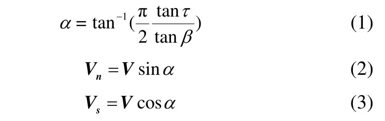
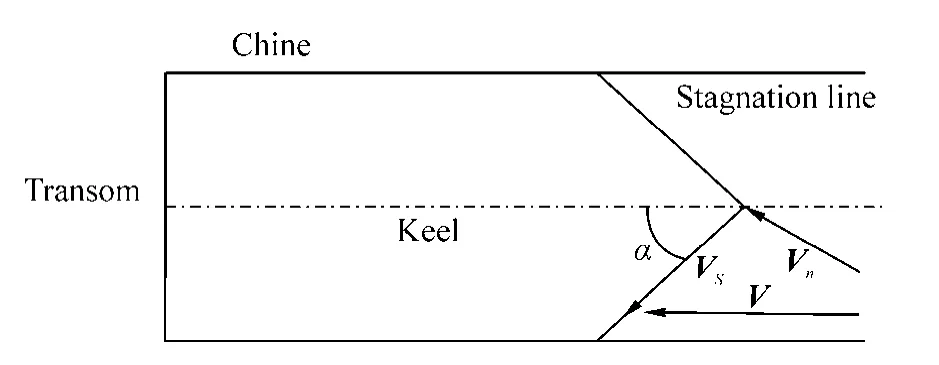
Fig. 1 Components of the velocity on the bottom of a planing hull using swept wing theory (Savitsky and Breslin,1958)

2.2 Spray apex theory

In a planing hull, the generated spray covering stagnation line leaves the hull from every point on the stagnation line.Whisker spray is part of the generated spray which transpires between the chine and stagnation line (Fig. 2). Main spray is seen as water particles reaching the chine. Therefore,projectile motion can be implemented for finding the trajectory of the spray. Lattore and Rayn (1989) attempted to use this method, but their assumption for spray velocity at the time of spray leaving the chine was erroneous as Morabito(2010) pointed out. Schematic of the spray motion and generation of the spray apex is illustrated in Fig. 2.

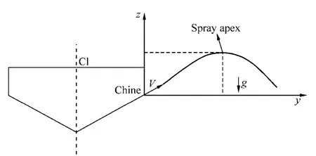
Fig. 2 Consideration of the projectile motion of the spray in transverse section (Morabito, 2010)

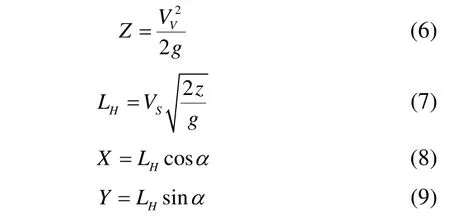
Savitskyet al.(2007) reported that spray velocity is equal to the velocity of the planing hull. Accordingly, it is sufficient to find the spray velocity in the direction ofz-axis as shown in Fig. 2. Savitsky and Morabito (2011) also used the swept wing theory to calculate the spray velocity and applied it to study projectile motion. Initially, they introduced spray velocity normal to the stagnation line.Afterwards, the angle between stagnation line and the horizon in transverse plane (βE) was defined as

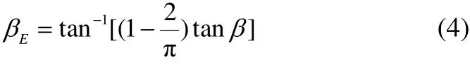
and an equation in the form of

was introduced for the vertical velocity of spray. Hence,spray apex will be obtained using the projectile formulation.The spray apex (Z), horizontal distance that spray travels before reaching apex (LH), and longitudinal (X) and transverse (Y) position of spray apex can be obtained using Eqs. (6) through (9).

2.3 Analytical solution

2.3.1 Geometrical equations

Several vectors are introduced by Morabito (2010) in order to investigate spray characteristics and a coordinate system is used in this regard. The intersection of the keel and calm water line is considered as the origin of this coordinate system, as shown in Fig. 3.

Three vectors are defined as follows (Morabito, 2010):

· SC: Vector along the spray root line, from keel to chine.The origin of this vector is the intersection of keel and calm water.

· KC: Vector from keel to chine. This vector represents the distance from keel to chine. Only the y-component andz-component of this vector are vital.

· KW: Vector from the intersection of keel to still water atx-location where the stagnation line crosses the chine. All these vectors are illustrated in Fig. 4.

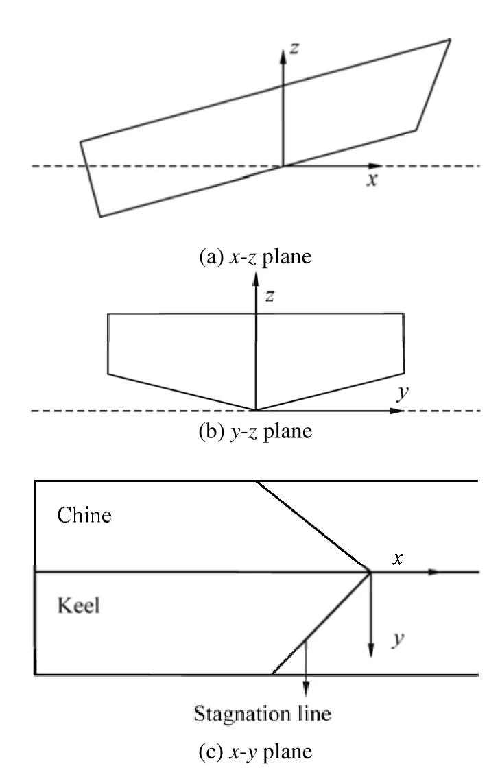
Fig. 3 Coordinate system

Fig. 4 Defined vectors (Morabito, 2010)

These three vectors can be calculated using geometry of the prismatic planing hulls. To accomplish this task,equations (10) through (15) were presented by Morabito(2010).

Morabito (2010) also used two other vectors to calculate the velocity; one being along the stagnation line (NIP) and the other normal to the stagnation line (NVD). These two vectors are:

· NIP: Vector normal to stagnation line in the plane of the hull.

· NVD: Direction vector of velocity normal to stagnation line.

These vectors are displayed in Fig. 5 and can be obtained using equations (16) through (21) (Morabito, 2010).

Fig. 5 Vectors NIP and NVD (Morabito, 2010)

Two components of velocity can be written as follows(Morabito, 2010):

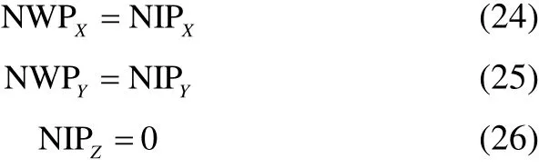
Furthermore, vectors which are found in the intersection of the normal plane and calm water are called intersection vectors and can be written in forms of equations (24) to (26)introduced by Morabito (2010):

Three angles were presented by Morabito (2010) which are used for modeling the spray and they are defined as:

·τNHW: Angle between the bottom of the hull and horizon in normal plan to stagnation line,

·τNVW: Angle between the normal velocity and horizon in normal plane to stagnation line,

·τNVH: Angle between the normal velocity and bottom of the hull in normal plane to stagnation line.

These angles can be obtained by means of dot product.Eqs. (27) through (29) are used for calculation of these angles.

Spray root geometry and position of spray in each section are required for computing the trajectory of the spray. By consideringl1as the distance between leading edge and stagnation line andl0as the distance between trailing edge and stagnation point, simple geometrical laws can be utilized for calculating the ratio between these two lengths in the geometry of the problem (Fig. 6) and equations (30) is introduced.

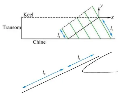
Fig. 6 Geometry of the spray root in the normal plane to the stagnation line (Morabito, 2010)

If the value ofl1is assumed to be equal to the distance between stagnation line and the keel, Eq. (31) can be written in the form of Eq. (32) and geometry of spray in each normal section can be calculated using Eqs. (33) through (35):

2.3.2 Green’s solution for the planing plate

Green’s solution (1936) plays a major role in the modeling of spray in planing hulls. By using this solution, a planing plate can be analyzed and lift coefficient, center of pressure as well as other characteristics of the planing plate can be obtained. In Green’s solution, position of the stagnation point is an important variable that affects the spray thickness and can cause a rotation in spray. Effects of this parameter on the spray can be observed in Fig. 2. By consideringτ'as the trim angle of the planing plate, the value of this angle in the modeling of the planing plate by Morabito (2010) becomes equal toτNVH. The ratio of the length of planing plate (distance from leading edge to the trailing edge) to the spray thickness can be calculated using the relation:

where

and parameterbranging from 1 to 3, expresses the position of stagnation point. By increasingbto 3, the stagnation point approaches the trailing edge. Rotation angle of the spray is established using Eq. (38) and ratiol1/lcan be calculated using Eq. (39).

where

2.3.3 Dynamical equations

By using Green’s solution (1936), there will be a set of angels for variousl1/lratios. Many of these values will be used in each section for calculating the velocity direction after reaching the chine. As spray approaches the chine, it leaves the hull with a specific angle which is calculated using Eq. (41), presented by Morabito (2010):

Therefore, normal velocity after rotation will be written i n the form of

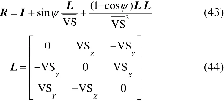
whereRis introduced by Morabito (2010) as follows:

The velocity with which the spray leaves the chine can be computed using summation of velocity vector along the stagnation line and vector of normal velocity after rotation as in

UsingVSRand the principle of projectile motion, spray trajectory can be attained as a function of time. The trajectory has the following formulation:

3 Computational algorithm

Mathematical modeling of spray using equations presented in Section 2 is possible, but not straight forward.For this reason, the current authors have designed a computational process which is the focal point and main aim of this article. The offered algorithm has two major parts. In the first part of the process, geometrical vectors, angles, and existing ratios in Green’s solution are calculated. In the second part, spray trajectory is modeled by the use of dynamic equations. Outputs of the first part are inputs for the second part. Computations in the first part are done in the following manner (as shown in Fig. 7):

1) SC, KW and KC are calculated using Eq. (10) through(15),

2) NIP and NVD are obtained using (16) through (21),

3) The velocity vectors are found at the third step using vectors in step (1) through (2),

4) NWP and three angles should be computed using their definitions and dot product,

5) Green’s solution is initiated after step 4),

6) Trim angle of the planing plate is set equal toτNHVcalculated in step 4),

7) By varyingbfrom 1 to 3, the following values are found:

·l/δas a function ofbanda

·γas a function ofbanda

·z/δas a function ofT

·l1/las a function ofT

8) Ifδ/l>gt;1 orδ/l>lt;0, then Green’s solution should be finished,

9) There will be a set ofγvalues for various stagnation points’ positions (δ/l>gt;1) in a planing plate with trim angle being equal toτNHV.

Fig. 7 The algorithm for obtaining Green’s solution and geometrical vectors and angles

In the second part of the designed algorithm (Fig. 8),normal planes to the stagnation line will be considered. From the first point where the spray is generated (x=−NIPX) to the last point where it still exists (x=SCX), the following calculation is done step by step for each section:

Fig. 8 The algorithm for mathematical modeling of three dimensional geometry of the spray

1) Calculating the spray root (POST),

2) Determining the ratio of the distance from the leading edge to stagnation line, to the distance from the trailing edge to the leading edge (l1/l), using Eq. (33),

3) Predicting value of the rotation angle at the desired section as follows:

· Ifl1/lis greater than all the values ofl1/lobtained in Green’s solution for planing plate with trim angle ofτNHV,there will be no rotation angle (because stagnation point has not approached the point where rotations begins)

· If the value ofl1/lcan be found in the range of values ofl1/lobtained from the Green’s solution , then interpolation should be applied for prediction ofγat the desired section

· If 0.98>lt;l1/l>lt;1, there is no need for interpolation and the rotation angle will be equal to π–τNHV(because spray has been rotated completely as represented by Green (1936))

4) Finding rotation matrix using Eq. (44)

5) Obtaining final velocity of the spray in each section(VSR)

6) Calculating the spray trajectory using Eq. (46) as a function of time. When the vertical position of the generated spray in the desired section approaches a negative number,solution process in that section is completed, because the spray generated by the section has reached the water surface.

7) By computing the required values in steps 1) through 6), there will be a spray trajectory in each section and by plotting trajectories together three dimensional geometry of the spray is obtained.

4 Validation

Results obtained using the suggested algorithm are compared with analytical equations of the spray apex, ie. Eqs.(6) through (9) which was presented in ref Savitsky and Morabito (2011). This validation is elected for a prismatic planing hull withβ=15°andB=22.86 cm. Position of the spray apex is the direct result of using an algorithm which searches the resulting trajectories of the PHSP code and the position of the point with maximum vertical positions. This will be compared with the equations and longitudinal, lateral and vertical components of spray apex. The accuracy of the position of spray apex will be investigated through different comparisons. With this in mind, various trim angles and speed coefficientsCV=2, 4 are considered as two variables for comparison purposes. Comparisons are done for non-dimensional position of spray apex (shown in Fig. 9)which can be calculated as follows:

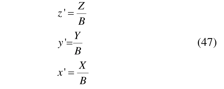
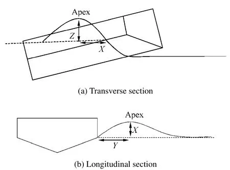
Fig. 9 Determination of apex position with respect to chine

Fig. 10 Comparison of the current results of the proposed algorithm against those by Eqs. (6) to (9), in a planing hull with β=15°and B=22.86 cm

Comparison of the results in different cases is illustrated in Fig. 10. Height of the spray apex using computational procedure is compared against the result of analytical equation (Savitsky and Morabito, 2011) in Fig. 10. Based on Figs. 10(c) and 10(f), it can be concluded that the results of the current algorithm and that of equation 6 are analogous. In Figs. 10(a) and 10(d), comparison of the results of the present algorithm and that of the analytical equation for longitudinal position of spray apex is displayed. As seen in these plots,results of the PHSP code and the analytical solution are similar, especially at trim angles greater thanτ=6°for both cases. Comparisons of the current results against those by Savitsky and Morabito’s equation (2011) for the lateral position of the spray apex are illustrated in Figs. 10(b) and 10(e). Agreement displayed by these plots confirms the accuracy of the developed code, albeit the results of the analytical equation by Savitsky and Morabito (2011) are slightly higher for the trim angles greater thanτ=6°.

5 Discussion of results

The obtained results are discussed in five major parts. In the first part, the effects of various physical parameters on the position of spray apex are studied. In the second part, an algorithm is added to Savitsky’s (1964) method to investigate variations of spray apex for a boat as a function of speed where trim angle and speed coefficient are varied as well. In the third part, a three dimensional geometry of the spray will be investigated. Finally, in the last two sections of this paper top and lateral views of the spray are studied.

5.1 Effects of physical factors

The first parameter considered is the deadrise angle of a planing hull. Effects of this factor is investigated for a prismatic planing hull withB=22.86 cm, trim anglesτ=2°, 4°,8°, 12°and two speed coefficients ofCV=2, 3. Results of these studies are illustrated in Fig. 11. As evident in this figure, in a planing hull with constant trim angle and speed coefficient,increasing the deadrise angle will cause a decrease in the height of spray apex, as shown in Figs. 11(a) and 11(d). For the hull withβ=40°and low trim angle (τ≤4°),non-dimensional height of spray apex approaches zero. On the other hand, non-dimensional longitudinal position of spray apex starts to increase and then decreases by reaching a specified deadrise angle which is between 10°to 20°. This fact can be seen in Figs. 11(c) and 11(f). This reduction depends on the trim angle. At greater trim angles, reduction occurs for smaller deadrise angle. Figs. 11(b) and 11(e)clearly show that non-dimensional longitudinal position of spray apex decreases with a decrease in deadrise angle, while all the parameters stay constant. It can be extrapolated from cases shown in Fig. 11 that speed coefficient affects the position of spray apex, i.e. greater value of speed coefficient(CV) will bring about a greater value for spray apex height(Figs. 11(a) and 11(d)) for longitudinal (Figs. 11(b) and 11(e))and for lateral position (11(c) and 11(d)) of spray apex.

As discussed before, speed coefficient is another effective parameter. In order to investigate the effects of this parameter for a planing hull withB=22.86 cm, at two deadrise anglesβ=20°, 30°and four different trim anglesτ=2°, 4°, 8°and 12°,the spray apex position is calculated. Fig. 12 shows the result of this case.

Results displayed in Fig. 12 show that an increase inCVwith the assumption that trim and deadrise angles are constant,causes an increase in height of spray apex (Figs. 12(a) and 12(d)). Figs. 12(b) and 12(e) show a similar variation trend in terms of lateral position of spray apex at four different trim angles (τ=2°, 4°, 8°, 12°). Longitudinal position of spray apex increases with an increase in the speed coefficient in both cases (Figs. 12(c) and 12(f)).

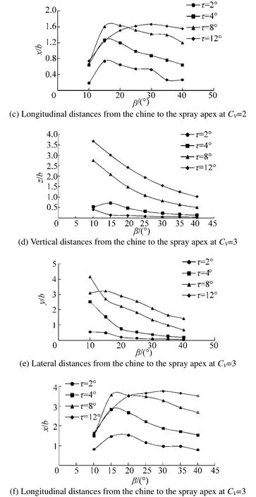
Fig. 11 Effect of deadrise angle in a planing hull with B=22.86 cm in various trim angles

In order to study the effect of the trim angle on the position of spray, the position of spray apex is obtained using the offered computational procedure. Two planing hulls with different deadrise angles ofβ=20°, 30°and similar beamsB=22.86 cm at two different speed coefficients ofCV=2, 4 are considered. Results are illustrated in Fig. 13. It is clear that an increase in trim angles when other factors are constant causes an increase in the height of spray apex for both planing hulls(Figs. 13(a) and 13(d)), but the slope of the resultant plot decreases in both the cases. This decrease can be observed beyondτ=15°. Effects of this parameter on lateral spray apex are different as shown in Figs. 13(b) and 13(e). The resultant of non-dimensional lateral position of spray apex increases until it reaches a specified trim angle from which a reduction will take place. For the case ofβ=20°, this trim angle is about 15°and for the caseβ=30°, this occurs after a trim angle of 30°. The non-dimensional longitudinal position of spray apex starts to increase when trim angle increases and other factors are kept constant, as shown in Figs. 13(c) and 13(f). As the non-dimensional position of spray apex decreases, there will be a decrease in longitudinal position, as well. This decrease is observed atτ=8°for the planing hull withβ=20°(Fig. 13(c))at both speed coefficients and atτ=15°for the planing hull(Fig. 13(e)) withβ=30°, at both speed coefficients.

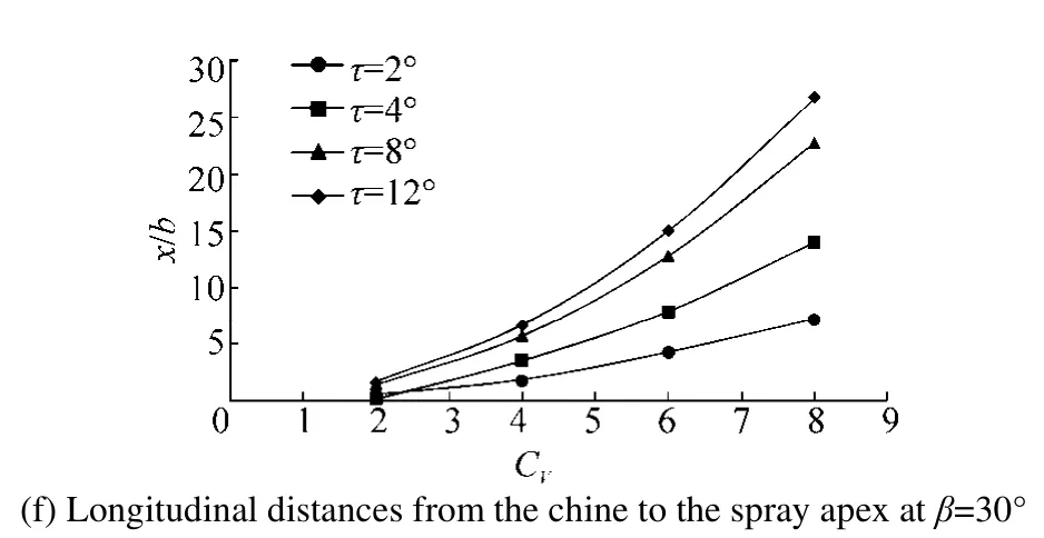
Fig. 12 Effect of speed coefficient in a planing hull with B=22.86 cm at various trim angles

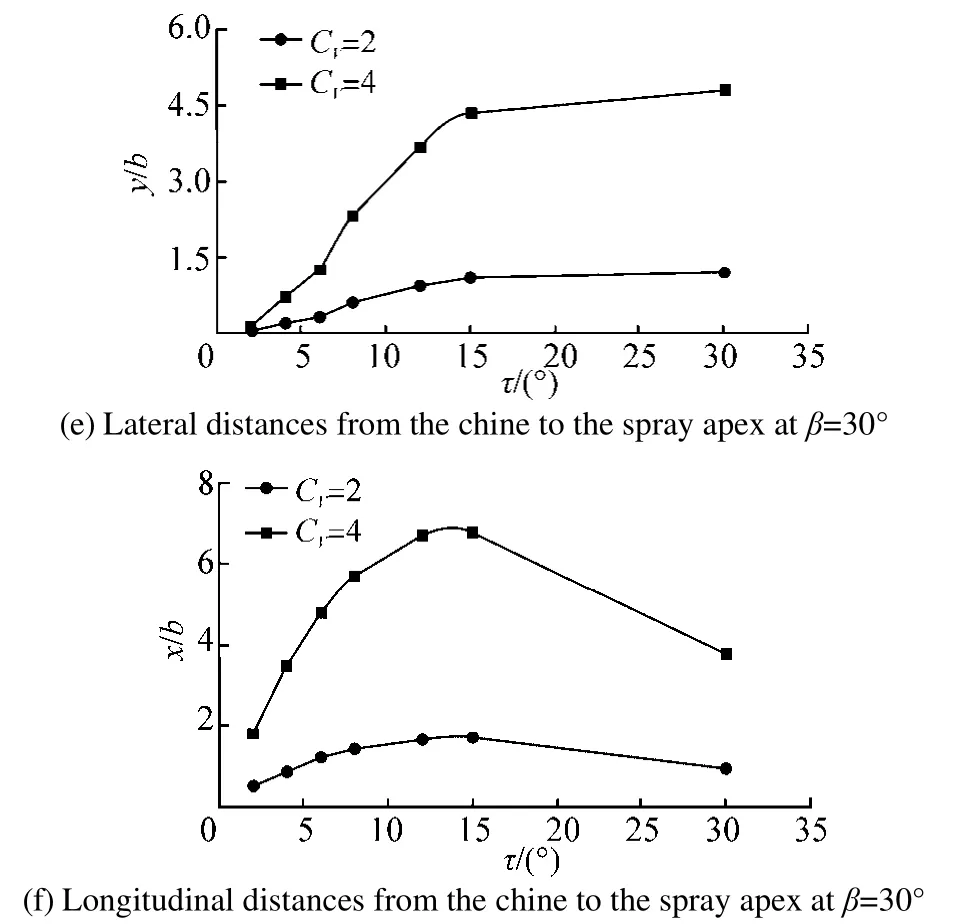
Fig. 13 Effect of trim angle in a planing hull with B=22.86 cm at various speed coefficients

5.2 Addition of proposed algorithm to Savitsky’s model

In order to obtain more useful results, the proposed algorithm is applied in conjunction with Savitsky’s (1964)method to model spray of a planing hull that possesses an increasing velocity. Savitsky’s (1964) procedure provides real characteristics of a planing hull including trim angle as well as other parameters. Therefore, the velocity of the planing hull is gradually increased and the trim angle and speed coefficient are calculated at each velocity. Subsequently, a variation of spray apex position for a planing hull that includes increasing velocity is computed and spray apex position can be plotted via the speed. A computer code has been developed for studying a prismatic planing hull with constant deadrise angle and beam. Characteristics of the considered hull are presented in Table 1. Figs. 14 and 15 demonstrate the obtained results for the trim angle and position of spray apex, respectively.

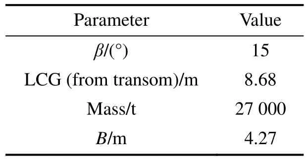
Table 1 Values of parameters considered in studying the planing hull

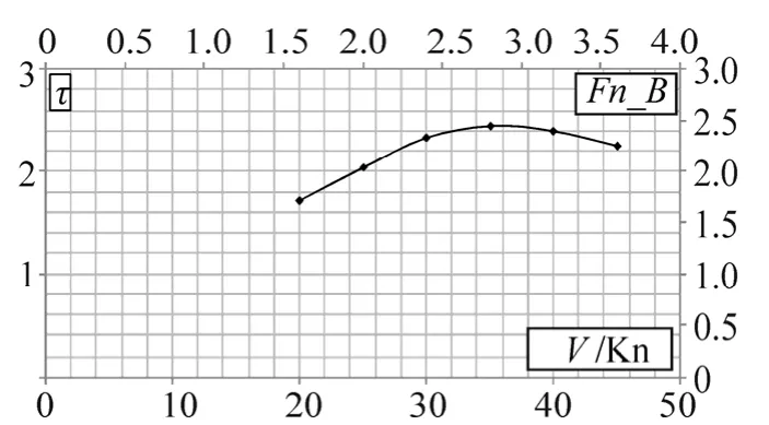
Fig. 14 Changes in trim angles as a result of increasing the speed in the considered planing hull

Fig. 15 Plots of dimensionless from the chine to the spray apex vs. speed in the considered planing hull

The results of this study clearly indicate that all three components of spray apex increase as the velocity of a prismatic planing hull increases. The main reason behind this behavior is the increasing in the speed coefficient of the boat.

5.3 Three-dimensional geometry of spray

Geometry of the spray is modeled using the above mentioned computational procedure. This geometry is studied for a planing hull withB=2 m,β=15°at four trim anglesτ=2°,4°, 6°and 8°and two different speed coefficients (CV=2, 4).The results are illustrated in Figs. 16 and 17. In all these cases,there is a flat sheet which is representative of the whisker spray. There is another conic pattern which is representative of the main spray that is generated in a small length of the chine. This geometry is comparable to the one discussed by Savitsky and Breslin (1958). These geometries indicate that an increase in the trim angle yields an increase in the volume under the main spray. Also, an increase in the spray apex in both described cases. The obtained geometries for high trim angles (i.e.τ=6°, 8°) atCV=4 seem unreasonable. This is because of the assumptions made for the mathematical modeling of spray. These assumptions include ignoring the surface tensions and aerodynamics forces.

Fig. 16 Three dimensional geometry of the spray in a planing hull with B=2 m, β=15°and CV=2

Fig. 17 Three dimensional geometry of the spray in a planing hull with B=2 m, β=15°and CV=4

5.4 Transverse view of spray

The trajectory over which the spray has maximum lateral distance from the chine has been simulated for two planing hulls withβ=15°, 30°andB=2 m at different trim angles.The results can be seen in Fig. 18. In both cases, the speed coefficient isCV=2. This figure confirms the fact that maximum lateral distance of the spray from the chine increases with trim angle, while height of the spray increases simultaneously.

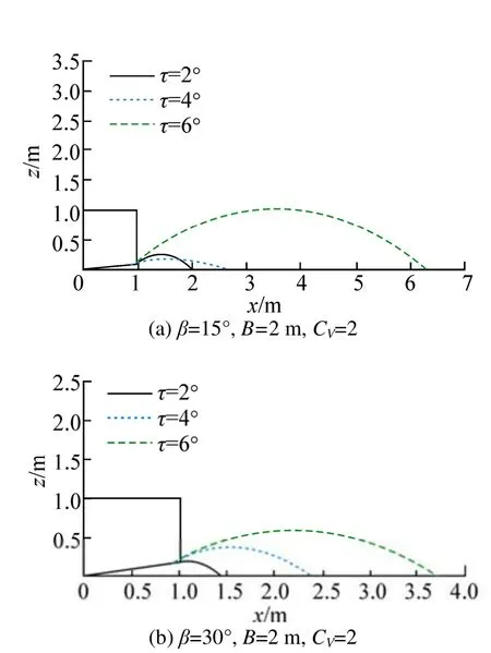
Fig. 18 Travelled trajectories by the spray which have maximum lateral distance from the vessels which is caused by the main spray at various trim angles

5.5 Top view of spray

The geometry of main spray in top view is considered as a characteristic of spray and can be used in hydrodynamic design of the planing hulls. Geometry of the spray in this view is like a triangle where one edge is the first trajectory travelled by the main spray and the second edge is the last trajectory travelled. The third edge is not similar to a line and is comparable to a curve, but is assumed to be like a line,as shown in Fig. 19. The angle between the first trajectory and the chine in top view (i.e.θf) and the angle between the last trajectory and the chine in top view (i.e.θl) have been defined and investigated here. Schematic of the geometry of the main spray with along with the mentioned assumption and the new angles are illustrated in Fig. 19. Initially, the effect of trim angle on the geometry in top view is found.Accordingly, the first and last trajectories as well as the other edge of the main spray on a planing hull withB=2 m andβ=15°at three trim angles are modeled and displayed in

Fig. 20. In this figure, intersection of the first and last trajectory is closer to the bow of the craft at greater trim angles andθfandθlboth increase as trim angle increases.The exact value of the defined angles is shown in Table 2.

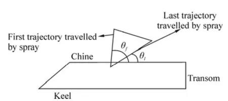
Fig. 19 Geometry of the main spray in top view

Fig. 20 Top view of the main spray at various trim angels in the planing hull with β=15°, B=2 m, CV=2

Fig. 21 Top view of main spray at various deadrise angles in the planing hull with τ=2°, B=2 m, CV=2

Table 2 Values of the defined angles in top view of the spray at various trim angles for the planing hull with β=15°, B=2 m, CV=2

Table 3 Values of the defined angles in top view of the spray at various trim angles for the planing hull with β=15°, B=2 m, CV=2

Variation of the geometry in top view has been established by studying two different cases. Both of these cases includes the same trim angle (τ=2°), speed coefficient(CV=2), and beam (B=2 m). Spray geometries are shown in Fig. 21 for two deadrise anglesβ=15°, 25°. This figure indicates that intersection of the first and last trajectory is closer to the transom atβ=25°and the defined angles are smaller in this case. The results of modeling at these angles are summarized in Table 3.

6 Conclusions

Using normal sections to the stagnation line and utilizing the swept wing theory is a particular approach for simulating the spray. In this way, several equations should be combined with each other. To accomplish this, an algorithm is designed and evaluated by comparing two existing analytical equations for the spray apex. This algorithm has two parts. In the first part in consists of vectors, angles, and Green’s solution are considered. Secondly, spray trajectory is determined in all sections using the results of the first part and principles of the projectile motion. By applying this algorithm, a detailed study is conducted and the following results are obtained:

1) If all parameters are kept constant except the deadrise angle that increases, the vertical distance of the spray apex from the free surface of the water increases. In this situation,there is an inverse relation between the deadrise angles and lateral and longitudinal distances from the spray apex to the chine. Initially, lateral and longitudinal distances of the spray apex from the chine increase by an increase in the deadrise angle. However, as they approach a specified trim angle between 20°and 30°they begin to reduce.

2) As the trim angles increase and other physical factors remain constant, the vertical position of the spray apex becomes greater, while the slope of the related plot decreases. In the cases in which the speed coefficient is smaller, the slope decreases at a greater rate. Longitudinal distance of the spray apex from the chine increases when the value of the trim angles increase, but it begins to decrease at the trim angle of 8°for the planing hull ofβ=20°. However,forβ=30°, it begins to decrease at the trim angle of 15°. For lateral distance, the trim angle is about 15 and 30 forβ=20°andβ=30°, respectively. It is therefore, concluded that decrease in trim angles is highly dependent on the deadrise angle and speed coefficient.

3) There is a direct relationship between the speed coefficient and position of the spray apex. Particularly, when the vertical, lateral, and longitudinal positions of the spray apex increase and when all the parameters are kept constant except for the speed coefficient that is increased.

All the presented equations prove that the wetted length of planing hull does not affect the spray because this parameter does not exist in any of the presented equations.For a more practical study, the proposed algorithm is added to the previously reported methods for performance prediction and changes of the spray apex position is investigated by increasing the velocity of the planing hull.The results from this study indicate that all the components of the spray apex increase as the velocity increases and the three obtained plots are in linear form.

Three-dimensional profiles of the spray are simulated by applying the proposed algorithm. The obtained geometry contains two patterns of spray that are similar to a flat sheet and a cone. This geometry proves that the suggested algorithm can model both patterns of the spray accurately.The main spray in the related figures is generated in a miniscule length of the chine as reported in the literature. As the trim angle increases, the volume under the surface of the spray gets larger. In the cases where the trim angle is greater than 6°and speed coefficient is equal and greater than 4,three dimensional profile of the spray seems unreasonable which is due to ignoring the surface tension effect.

Transverse view of the spray is also studied and the trajectory over which the maximum lateral distance from the chine occurs is plotted. The results of this study proved that increasing the trim angle causes an increase in the maximum lateral distance.

Finally, geometry of the spray in top view is modeled and two new angles are defined. It is observed that these two angles begin to increase as trim angles increase and all the factors are kept constant while the intersection of the first and last trajectory of the main spray moves towards the bow of the hull. Changes in this geometry are investigated when deadrise angle varies and it is found that the intersection gets closer to the transom stern and both of the defined angles get smaller, as this parameter increases.

Nomenclatures

aA parameter in Green’s solution

AA constant in Green’s solution

bA parameter in Green’s solution

BBeam

CVSpeed coefficient

gAcceleration due to gravity

IIdentity matrix

KC Vector from keel to chine - this vector represents the distance from keel to chine–only KCyand KCZare needed

KW Vector from intersection of keel to steel water atx-location where stagnation line crosses the chineonly KWyand KWZare needed

lDistance from trailing edge to leading edge in Green’s solution

l0Distance from stagnation line to leading edge in Green’s solution

l1Distance from trailing edge to stagnation line in Green’s solution

LA defined matrix for calculation ofR

LHHorizontal distance spray travels before reaching apex

LCG Longitudinal center of gravity

NIP Normal vector to stagnation line in the plane of hull,including NIPX, NIPYand NIPZ

NVD Direction vector of velocity, normal to stagnation line, including NVDX, NVDYand NVDZ

NWP Intersection Vector (intersection of normal plane and the water)

POSTPosition vector of spray root in each section, normal to stagnation line,including POSTX, POSTYand POSTZ

PS Position of spray at each section, as a function of time (spray trajectory), including PSX, PSYand PSZ

RRotation matrix

SC Vector along spray root line from keel to chine,Including SCX, SCYand SCZ

tTime

TA variable in Green’s solution for calculatingl1/l.T=0, −1, 1,a

USpeed of planing plate in Green’s solution

VVector velocity of planing craft

VnVelocity component of planing hull normal to the stagnation line

VSVelocity component of planing hull along the stagnation line

VSRResultant velocity of spray

VSVVertical component ofVSin transverse plane

VN Normal velocity vector to stagnation line

VNRNormal velocity after rotation

VS Velocity vector along the stagnation line

xLongitudinal distance from intersection of keel and normal sections to the coordinate origin

XLongitudinal Component of spray apex

x'X/B

YLateral component of spray apex

y'Y/B

ZVertical component of spray apex

z'Z/B

αAngle between stagnation line and keelβDeadrise angle

βEAngle between stagnation line and horizon in transverse plan

γRotation angle of spray in Green’s solution

δSpray thickness in Green’s solution

θfAngle between first trajectory and chine inxyplane

θlAngle between last trajectory and chine inxyplane

τTrim angle

τ'Trim angle in Green’s solution

τNHWAngle between bottom of the hull and horizon in normal plan to stagnation line

τNVHAngle between normal velocity and bottom of the hull in normal plane to stagnation line

τNVWAngle between normal velocity and horizon in normal plane to stagnation line

ψRotation angle of velocity normal to stagnation line

Green AE (1935). The gliding of a flat plate on a stream of finite depth part I.Mathematical Proceedings of the Cambridge Philosophical Society, 31, 584-603.

Green AE (1936). The gliding of a flat plate on a stream of finite depth part II.Mathematical Proceedings of the Cambridge Philosophical Society, 32, 67-85.

Kihara H (2006). A computing method for the flow analysis around a prismatic planing hull.5th International Conference on High Performance Marine Vehicles, Tasmania, Australia, 262-272.

Kikuhara S (1960). A study of spray generated by seaplane hulls.Journal of the Aero-Space Science, 27(6), 415-428.

Lattore R, Ryan S (1989). Dimensional and similitude analysis of spray blister sheet from prismatic planing models.Ocean Engineering, 16(1), 71-83.

Locke FWS (1943).A method for making qualitative studies of the main spray characteristics of flying-boat hull models. Davidson Laboratory, Hoboken, United States, Report No. 232.

Morabito MG (2010).On the spray and bottom pressure on planing surfaces. PhD thesis, Stevens Institute of Technology, Hoboken,United States.

Payne PR (1986). On the spray sheet thickness of a planing wedge hull.Ocean Engineering, 13(1), 1-36.

Payne PR (1989). Dimensional and similitude analysis of spray blister sheet from prismatic planing model.Ocean Engineering,16(1), 71-83.

Pierson JD, Leshnover S (1950).A study of the flow, pressures, and loads pertaining to prismatic vee-planing surfaces. Davidson Laboratory, Hoboken, United States, Report No. 382.

Savitsky D (1964). Hydrodynamic design of planing hulls.Marine Technology, 1(1), 71-95.

Savitsky D, Breslin J (1958).On the main spray generated by planing surfaces. Davidson Laboratory, Stevens Institute of Technology, Hoboken, United States, Report No. 678.

Savitsky D, DeLorme MF, Datla R (2007). Inclusion of whisker spray in performance prediction method for high speed planing hulls.Marine Technology, 44(1), 35-67.

Savitsky D, Morabito MG (2011). Origin and characteristics of the spray patterns generated by planing hulls.Journal of Ship Production and Design, 27(2), 63-83.

Sottorf W (1932).Experiments with planing surfaces. NACA Technical Memorandum, No 739.

Wagner H (1932).Phenomena associated with impacts and sliding on liquid surfaces. NACA Translation.

Zarnick EE (1978).A non-linear mathematical model of motions of a planing boat in regular waves. David Taylor Naval Ship Research and Development Center, Bethesda, United States,Technical Report No. DTNSRDC-78/032.