Experience Replay for Least-Squares Policy Iteration

Quan Liu Xin Zhou Fei Zhu Qiming Fu Yuchen Fu

I.INTRODUCTION

R EINFORCEMENT learning(RL)interactsw ith the environmentand learnshow tomap situations to actions in order to obtainmaximum cumulative reward.Agents constantly try to find the bestaction which gets themaximum reward.In reinforcement learning cases,theactionw illnotonly affect the immediate rewards,butalso the next state and all subsequent reward.Reinforcement learning is characterized by trial and error search as well as delayed reward[1−2].Reinforcement learning has good learning performance in complex nonlinear systems w ith large spaces,and is w idely used in process control,task scheduling,robotdesign,gam ing andmany other fields[3−5].

In reinforcement learning,we use the value function to estimate the long-term cumulative reward ofa stateor state-action pair.The V-function estimates the state and the Q-function estimates the state-action pair.The policy in reinforcement learning is amapping from the state space to the action space,

Quan Liu is w ith the School of Computer Science and Technology,Soochow University,Jiangsu 215006,China,and also w ith the Key Laboratory of Symbolic Computation and Know ledge Engineering ofM inistry of Education,Jilin University,Changchun 130012,China(e-mail:quanliu@suda.edu.cn).

Xin Zhou is w ith the School of Computer Science and Technology,Soochow University,Jiangsu 215006,China(e-mail:504828465@qq.com).

Fei Zhu isw ith the Schoolof Computer Science and Technology,Soochow University,Jiangsu 215006,China,and also w ith the Key Laboratory of Symbolic Computation and Know ledge Engineering ofM inistry of Education,Jilin University,Changchun 130012,China(e-mail:zhufei@suda.edu.cn).

Qim ing Fu and Yuchen Fu are w ith the School of Computer Science and Technology,Soochow University,Jiangsu 215006,China(e-mail:fqm 1@126.com;yuchenfu@suda.edu.cn).agentseventually reach the target through comparing the value functions to seek the optimal policy[6].Policy iteration(PI)is an important reinforcement learningmethod,whosealgorithms update the currentpolicy by calculating thevalue functionsand then improve the policy w ith the greedy policy.Least-squares method can be used advantageously in reinforcement learning algorithms.Bradtke etal.proposed the least-squares temporal difference(LSTD)algorithm based on the V-function[7−8].Although their algorithm requiresmore computation cost for each time step,which is different from traditional temporaldifference(TD)algorithms,itcan extractmoreuseful information from theempiricaldataand therefore improve thedatavalidity.However,as the absence of model in action selection in the model free cases,LSTD only intended to solve the prediction problems,and could notbe used in the control problems[9−11].Lagoudakis et al.extended it to the least-squares temporal difference for Q-functions(LSTD-Q)[12−13],and proposed the least-squares policy iteration(LSPI)algorithm whichmade it available for control problems.LSPIused LSTD-Q in policy evaluation,and accurately estimated the current policy w ith all samples collected in advance,which was a typical offl ine algorithm.Reinforcement learning is capable of dealing w ith the interaction w ith the environmentonline.Busoniu etal.extended theoffl ine least-squarespolicy iteration algorithm to the online cases[14],and presented an online least-squares policy iteration(online LSPI)algorithm.The algorithm uses samples generated online w ith exploratory policy,and improves the policy every few steps.But it uses empirical data only once,which have low empirical utilization rate.Therefore,in the early time of the algorithm implementation,as there is few sample data available,it is difficult to obtain good control policy,which leads to poor initial performance and slow convergence speed of the algorithm.

Experience replay(ER)methods can reuse prior empirical data and therefore reduce the number of samples required to get a good policy[15],which generates and stores up sample data online,and then reuses the sample data to update the current policy.In this work,combining the ER method w ith the online LSPI,we propose an ER for least-squares policy iteration(ERLSPI)algorithm which is based on linear leastsquares function approximation theory.The algorithm reuses the sample data collected online and extractsmore information from them,leading to the empirical utilization rate and the convergence speed improvement.

II.RELATED THEORIES

A.Markov Decision Process

A state signal which retains all pertinent information successfully is supposed to have the Markov property.In reinforcement learning,ifa statehas theMarkov property,then the response of the environmentat timet+1 depends only on the representation of the stateand action at timet.A reinforcement learning task thatsatisfies theMarkov property is known to be aMarkov decision process(MDP).An MDP can be defined as the follow ing four factors:the state spaceX,the action spaceU,the transition probability functionf,the reward function

ρ.In the determ inistic case,the state transition function isf:X×U→[0,1],and the reward function isρ:X×U→R.At the current time stepk,the controller takes actionukaccording to the control policyh:X→Uin the given statexk,rk+1=ρ(xk,uk).In the stochastic case,the state transition function is:X×U×X→[0,∞),and the reward function is:X×U×X→R.At the current time stepk,the controller takes actionukaccording to the control policyh:X→Uin the given statexk,transfers to the next statexk+1(xk+1∈Xk+1,Xk+1⊆X)w ith the probabilityP(xk+1∈X k+1|xk,uk)=∫X k+1f(xk,uk,x′)dx′,and the system obtains the immediate rewardrk+1=(xk,uk,xk+1).If the state space is countable,the state transition function can bew ritten as:X×U×X→[0,1],the probability of transfer to the next state isP(xk+1=x′|xk,uk)=(xk,uk,x′).Givenfandρ,aswell as the current statexkand the current action takenuk,it issufficient to determ ine the nextstatexk+1and the immediate rewardrk+1,this is theMarkov property.It is the theoretical basis for reinforcement learning algorithms.

If an MDP has a term inal state,once it reaches the term inal state,it cannot transfer out,ofwhich task is called an episodic task;on the contrary,a task w ithout a terminal state is called a continuous task.In particular,an MDPw ithout unreachable states,w ith nonzero probability being accessed for each state is ergodic.

B.Online Least-Squares Policy Iteration

The Q-functionQhgiven by the policyhcan be found by solving the Bellman equationQh=Th(Qh),where the policy evaluation mappingThis[Th(Q)](x,u)={ρ(x,u,x′)+γQ(x′,h(x′)}.The PIalgorithm startsw ith an arbitrary initial policyh0,in each iterationl(l≥0),the algorithm evaluates the current policy,calculates the Q-function Qh l,and then useshl+1=argmaxuQh l(x,u)to improve the policy.The PI algorithm eventually converges to the optimal policyh∗.

Traditional algorithms exactly store the distinct value functions for every state(if V-functions are used)or for every state-action pair(in the case of Q-functions)w ith tabular method.When some of the state variableshave a very large or infinite number of possible values,determ ining exact storage is impossible,and the value functions have to be represented approximately.

In function approximation methods,we suppose the state spaceXand action spaceUcontain a finite number of elements,represented byX={x1,···,x}andU={u1,···,u},respectively.Define the basis function matrixφ∈Rn s×nas follows:

wherenis the dimension of the basis functions,lsis the serial number of samples,andnsis the number of samples.The basis functions are state-dependent.In the state-action basis function vectorφl(xls,uls),all the basic functions thatdo not correspond to the current discrete action are taken to be equal to 0:

whereφi(xls)(i=0,1,···,)is the Gaussian radial basis functions(RBFs),which can be defined as

whereµi(i=1,···,¯N)is the center of thei-th RBF andσis the w idth.

In linear parametric conditions,according to the basic functionφ,for a given policy parametersθ(θ∈Rn),approximation Q-functions can be represented by(2).

LSPI algorithm iteratively updates the policy parameterθto get the optimal policy.To find an approximate Q-functions for a policyh,a projected form of the Bellman equation can be w ritten as

wherePwperformsaweighted least-squares projection on the space of representable Q-functions[14].The projectionPwis defined by

where

LSPIalgorithm uses LSTD-Q to calculate the policy parametersθbased on all samples collected in advance,as follows:

wherematrixΓ,Λ∈Rn×n,and vectorz∈Rn.Γ,Λ,andzare defined as follows:

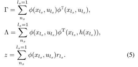
LSPI is an offl ine algorithm,all samples collected in advance are needed in each updating step.In online LSPI,the policy improvementsmustbe performed after several(not too many)steps(for continuous tasks)or episodes(for episodic tasks),and then applied to generate new samples.Then another policy improvement takes place,and the cycle repeats[14].

III.ER LEAST-SQUARES POLICY ITERATION

A.ER Least-Squares Policy Iteration

In the online LSPI algorithm,the sample data generated online is used only once and then be discarded,which leads to the low empirical utilization rate of the algorithm,especially in the cases where collecting samples is difficult.As a result,improving the empirical utilization rate is particularly important.In this work,we use the ER algorithm to achieve the goal.The sample data generated online is preserved for future reusing.The sample data is stored in the form of tetrad(x,u,r,x′),wherexis the currentstate,uis theselected action under current policy,ris the immediate reward obtained,andx′is the next state transferred to.The sample data constitute the experience,together w ith the current policyhconstitute the quintuple(x,u,r,x′,h(x′))to update policy.The policyhis associated with the policy parametersθ;differentθis corresponding to differenth;andh(x′)represents the action to be taken in statex′.Policy updating is performed after the prescribedkepisodes(episodic task)orTtime steps(continuous task)rather than after each time step.The entire sample data currently collected is used in each updating of the policy parameterθ,resulting in the updating of thecorresponding policyh,then the sample data is reused to constitute new quintuples to updateθunder the new policy.This procedure is executed repeatedly fordtimes to achieve the reuseofexperience.The sample collection is restarted after each update,which can prevent the happening of excessive sample data and the resulting excessive computational cost.

LSTD-Q is utilized to estimate policy,the calculation ofθby(4)requires to a complete matrix inversion,which is computationally intensivew ith high computational cost.Many approaches can beused to reduce the computation cost.In this work,we take advantage of the Sherman-Morrison approach to calculateθincrementally[7].SetmatrixB∈Rn×nw ith initialmatrixB0which is typically set as a diagonalmatrix of the formβΓI,whereβΓis a small positive constant,andIis an identitymatrix.This ensures thatB0is approximately 0,but is invertible.Suppose the serial number of the sample currently being processed isls,thenB lsis updated by:

So,through updating matrixBrecursively,the procedure ofmatrix inversion is om itted,and the computation is greatly reduced.The ERLSPI algorithm w ith LSTD-Q is showed as A lgorithm 1.

A lgorithm 1.ERLSPIw ith LSTD-Q

1:B=βΓI(βΓis a small positive constant)

2:z=0

3:ns=0(ns=0 is the number of current samples)

4:i=0(iis the counter)

5:Atcurrentstatexls,choose actionuls(ls=1,2,···)according to a certain policy(for exampleε-greedy)

6:Execute actionuls

7:Save sample data〈xls,uls,rls,x′ls〉

8:ls=ls+1

9:ns=ns+1xlsis the term inal state of episodek(for episodic task)

10:h(x′ls)=argm axuφT(xls,u)θls=1

12:ls=ls+1

un til:ls=ns

14:i=i+1

un til:i=d

15:ls=0

16:ns=0

17:i=0

un til:satisfy the term inal condition

The least-squares policy evaluation for Q-functions(LSPEQ)proposed by Jung et al.uses a formula sim ilar to(4)to process sample data to estimate policy[16−17].The initial parameter vectorθ0can be setarbitrarily.The updating equation is as follows:

Unlike ERLSPIw ith LSTD-Q,ERLSPIw ith LSPE-Q updates the policy parameterθaftereach state transaction,the updating is dependent on the results of the last step,so the value ofθis relevant w ith the order for samples processing.A lso,the updating is also affected by the step size parameterα.The algorithm is less stable than the ERLSPIw ith LSTD-Q which uses all samples currently collected and elim inates the step size parameterα.However,if a good initial value is given,by lowering the step size parameterαgradually,the algorithm can often achieve better performance.ERLSPIw ith LSPE-Q is given as A lgorithm 2.

Algorithm 2.ERLSPIw ith LSPE-Q

1:B=βΓI(βΓis a small positive constant)

2:z=0

3:ns=0(ns=0 is the number of current samples)

4:i=0(iis the counter)

5:rep eat

6:Atcurrentstatexls,choose actionuls(ls=1,2,···)according to a certain policy(for exampleε-greedy)

7:Execute actionuls

8:Save sample data〈xls,uls,rls,x′ls〉

9:ls=ls+1

10:ns=ns+1

11:ifxlsis the terminal state of episodek(for episodic task)

12:rep eat

14:ls=1

15:rep eat

16:

20:ls=ls+1

21:un tills=ns

22:i=i+1

23:un tili=d

24:ls=0

25:ns=0

26:i=0

27:en d if

29:un til satisfy the term inal condition.

B.Algorithm Analysis

To ensure the convergence of the algorithm,the samples must be generated w ith exploratory policies.If only stateaction pairs of the form(x,h(x))are collected,then the information of state-action pairs(x,u)is not to obtain whenu/=h(x)whichmeans the correspondingweightw(x,u)is0.Therefore,theQ-valuesof such state-action pairswould notbe properly estimated,or the improvementof approximation policy could notbewell performed according to Q-functions.To avoid this,in certain conditions,actions different fromh(x),such as random actions according to a certain probability,should be selected.For a given steady exploratory policy,the algorithm can be used to evaluate further exploratory policy.

Lemm a 1.For any Markov chain,if:1)θtis obtained by ERLSPI algorithm,2)each state-action pair(x,u)is visited infinitely,3)each state-action pair(x,u)is visited inproportion w(x,u)w ith probability 1 in the long run,4)and φTw(I−γ¯fh)φis invertible,then the equation

holds w ith probability 1,whereis the basis function matrix whose column x isis a diagonal matrix w(x,u),which represents the weight of state-action pair(x,u)andis amatrix of state transition probability andis a matrix about policy,when i′=i and h(xi)=uj,hi′,[i,j]=1,otherw iseis a vector about expected immediate reward and

Proof.In the case of online LSPI,at time t,by(4)we get

In the case of ERLSPIwhere the sample data w ill be reused d times,it can be further transformed into

When t→ ∞,according to condition 2),each state-action pair(x,u)is visited infinitely,and the transition probabilities of state-action pairs approach their true transition probabilityw ith probability 1.Meanwhile,by condition 3),each stateaction pair(x,u)is visited in proportion w(x,u)w ith probability 1.Therefore,by condition 4),theθERLSPIof ERLSPI can be estimated as

Theorem 1.For ergodic Markov chains,which have no unreachable states and each state is being accessed w ith nonzero probability,if:

1)The feature vectors{φ(x,u)|x ∈ X,u ∈ U}which represent state-action pairs are linearly independent,

2)The dimension of each feature vectorφ(x,u)is n=|X|×|U|,

3)The discount factor is 0≤γ＜1,then,when the state transition frequency tends to be infinite,the asymptotic parametersθERLSPIof ERLSPI algorithm converges to its optimal valueθ∗w ith probability 1.

Proof.As it is for ergodic Markov chains,when the time step t tends to be infinite,the frequency of each state-action pair approaches infinity w ith probability 1.Meanwhile,each state-action pair is visited in the proportion w(x,u)w ith probability 1,and for any(x,u)∈(X×U),w(x,u)＞0.Thus,the matrix w is reversible.By condition 2),φis a n×n squarematrix,and by condition 1),the rank ofφis n,thereforeφis invertible.By condition 3),0≤γ＜1,I−γ¯fh is reversible.Therefore,by Lemma 1,equationθERLSPI=[φTw(I−γ¯fh)φ]−1[φTw¯r]holdsw ith probability 1.

The Q-function satisfies the consistency condition:

So the expected immediate reward(x,u)can beattained as

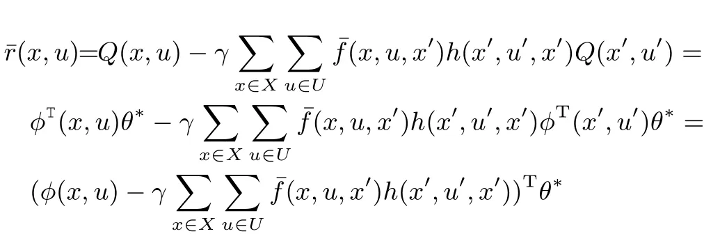
Itsmatrix form is

Substituting in the formula ofθERLSPI,we can get

Thus,θERLSPIconverges to θ∗w ith probability 1.

As the sample data is generated w ith an exploratory policy,each state-action pair(x,u)can be visited infinitely when t→ ∞,according to the law of large numbers,the probabilities of events happening approach their true probabilities,so the state transition probabilities between state-action pairs is an approximation to the true state transition probabilities¯f.Besides,the probability of being visited for each state-action pair(x,u)approaches w(x,u)w ith probability 1,whichmeets the ergodic Markov chain.Therefore,using the linearly independentGaussian radialbasis functionφ(x,u)(x∈X,u∈U)encoding whose dimension is n=|X|×|U|,and take the discount factor 0≤γ＜1,by Theorem 1,ERLSPIalgorithm converges.

From the pointof view of calculation,to calculateθdirectly by(3)requires to complete the operation ofmatrix inversion whose order of complexity is O(n3)where n is the dimension of radial basis functions.For episodic tasks,suppose that batch updating interval has k episodes,the sample data is reused d times,and the number of samples collected in an updating interval is m.In ERLSPI w ith LSTD-Q,θis calculated for d times in each updating interval,the average time complexity of each episode isin ERLSPI w ith LSPE-Q,θis updated once in every state transition,its time complexity isTo calculate incrementally by the Sherman-Morrison formula,the matrix inversion process is elim inated,the time complexity of each episode w ill be reduced toThe time complexity is proportional to d and is inversely proportional to k.The larger the value of k,the more experience is reused;the more quickly the optimal policy attained,the greater the computational cost is required.Thereby,we can reduce the number of the updating of policy by increasing the value of k properly,which can reduce the computational costs w ithout reducing the number of sample data.The time complexity of online LSPI,ERLSPI w ith LSTD-Q and ERLSPIw ith LSPE-Q are given in Table I.

IV.EXPERIMENT AND RESULTS ANALYSIS

A.Experimental Description

In order to verify the performance of the proposed algorithm,in thiswork we simulate the experimentof the inverted pendulum system,where,in a horizontal rail,there is a cart w ith an inverted pendulum which can move around,and the inverted pendulum can rotate about the axis freely w ithin the track,w ith thegoalof keeping the inverted pendulum balanced by applying different forces,as showed in Fig.1.

Fig.1. Inverted pendulum system.

According to[13],the state space of the system is continuous,the state space of the system,represented by the angleχbetween the inverted pendulum and the vertical direction and the currentangular velocity˙χ,is continuous.The action is the force applied to the cart,there are three distinct actions:leftward force(−50N),rightward force(50N),w ithoutapplying force(0N).All the three actions are noisy,a uniform noise in the interval[−10,10]is added to the selected actions,the actual(noisy)force applied to the cart is denoted byF,the transitions are governed by nonlinear dynam ics of the system which can be represented by

wheregis the acceleration of gravity(g=9.8m/s2),ais themass of the inverted pendulum,bis themass of the cart(b=8.0kg),lis the length of the inverted pendulum,andηis a constant(η=1/(a+b)).The time step of system simulation is 0.1s.This is an episodic task,as long as the absolute value of the angle between the inverted pendulum and the vertical direction doesnotexceed,the reward is0;otherw ise,once itexceeds,itmeans theend ofan episodeand getsa reward of−1.The discount factor of the experiment is 0.95.

B.Experimental Settings

In this experiment,for each action a set of 10-dimensional(30-dimensional w ith 3-actions)basis functions is used to approximate the value function,including a constant and 9 Gaussian radial basis functions in the two-dimensional state space.For the statex(χ,)and actionu,the basis functions corresponding to the remaining actions are all 0.The basis functions corresponding to actionuare as follows:

where inµi(i=1,···,9)is the grid pointof the two-dimensional state space andσis the variance.The number of m inimum balancing steps isset to 3000.Thatis,if the inverted pendulum does not fall after running 3000 time steps,this simulation can be considered to be successful,and the next episode starts.The maximum episode number of the experiment is set to 300.We analyze the performance of the algorithm by observing the balancing steps in 300 episodes.We useεgreedy as behavior policy in the experiment.The exploration probability is initially set to a valueε0=0.005,and itdecays exponentially once every second w ith rateεd=0.995.

wheresis the time steps,Tsis the number of sampling time of the process,Ts=0.1 s,and「.」denotes the floor operator.

C.Experimental Results and Analysis

The experimental results of online LSPImethod and ERLSPI w ith LSTD-Q under different parameters are shown in Fig.2,where the horizontal axis represents the episodes of the simulation experiment,the vertical axis represents the balancing steps in each episode of the inverted pendulum,drepresents thenumberofexperience reuse andkrepresents the updating interval.For example,in ERLSPI,k=5 andd=2 denoting the policy is updated once every five episodes and the experience is reused two times in each updating.In Fig.2(a),show ing results of ERLSPI(d=2),ERLSPI(d=5)and the online LSPI in the case ofk=1,the experimental data are the average results after running 10 times.Aswe can see from the figure,the balancing steps of online LSPImethod w ithin the fi rst 200 episodes are at a low level until about 230 episodes.The balancing stepsof ERLSPIare significantly larger than online LSPImethod,and the greater thedis,the more improvement we can get.The greaterdmeans more experience can be reused,the faster learning speed to the optimal policy,and the higher computational costs.Increasing the value ofkproperly can reduce the number of updating,which can reduce computational costs in the casewhen sample data is not reduced.In Fig.2(b),we can see whenk=5 where ERLSPI methods yield has good effects,the initial performance is slightly lower than those yielded byk=1.However,increasing the parameterkcontinuously only leads to gradual deterioration of experimental results,as shown in Fig.2(c).Therefore,appropriate parametersshould beselected to ensureexperimental resultsw ith proper computational costs.

Table II shows the balancing steps of online LSPI and ERLSPIw ith LSTD-Q under different parameters in the fi rstp(p=50,100,150,200,250,300)episodes.Data in Table II shows that,the balancing steps of online LSPI w ithin the fi rst 200 episodes have been smaller than 50 steps,which eventually reach 2112 stepsw ithin the 300 episodes,while the balancing steps of ERLSPI,d=5 are up to several hundred in dozens of episodes,and finally reached the 3000 balancing steps in 300 episodes.Therefore,reusing previous experience can significantly improve the performance of the algorithm,and improve the convergence speed.

TABLE I THEORDER OF TIME CPOMPLEXITY OFONLINE LSPI,ERLSPIW IRH LSTD-Q AND ERLSPIW ITH LSPE-Q

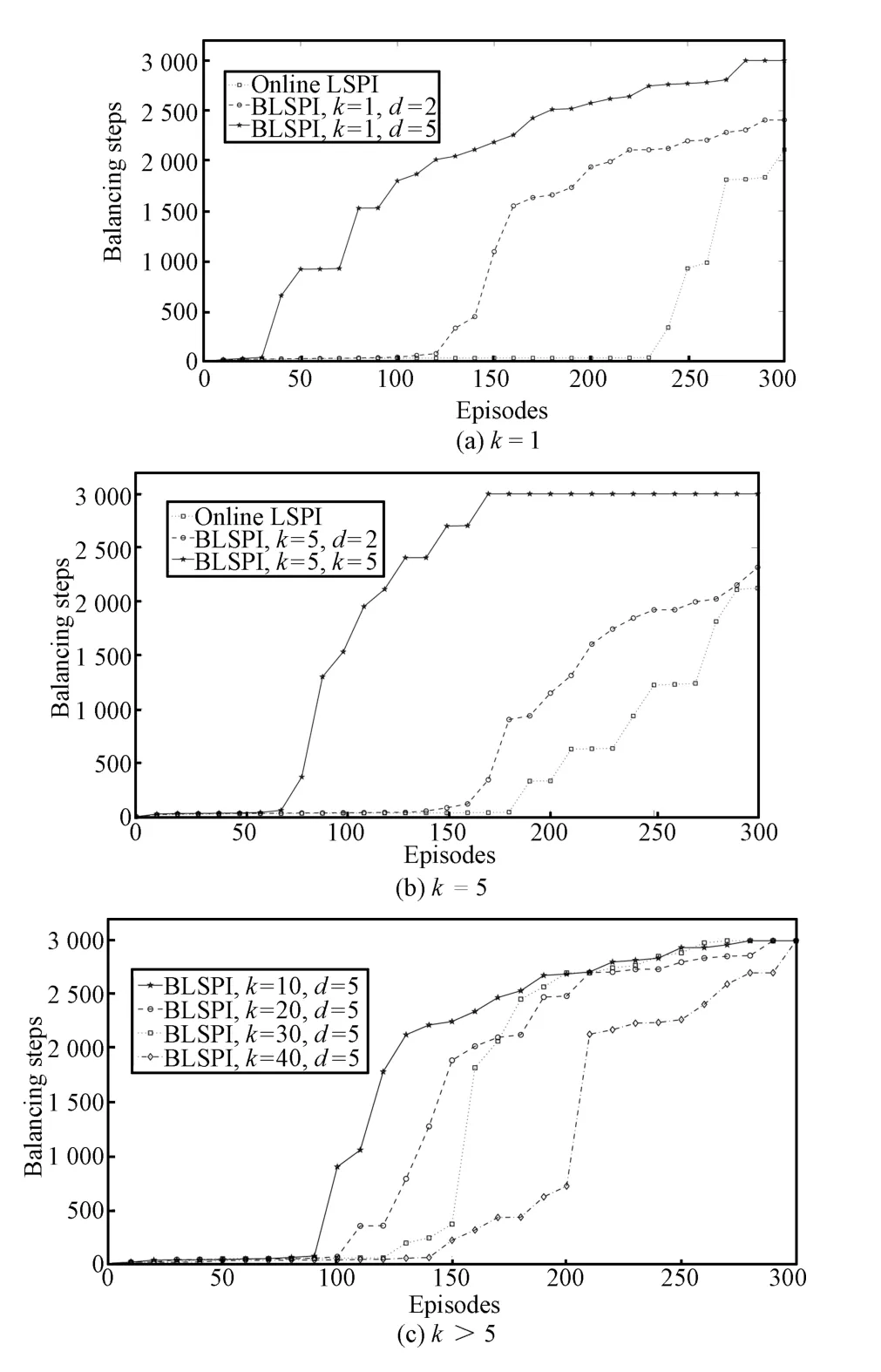
Fig.2. The performance of online LSPIand ERLSPIw ith LSTD-Q under different parameters.

In the case ofk＞5,whenkincreases,the computational costs become smaller and smaller,and so are the balancing steps,but they still reach 3000 balancing steps w ithin 300 episodes.

The experimental results of online LSPIand ERLSPIw ith LSPE-Q under differentparametersare shown in Fig.3,where the step size parameterα=0.005.In Fig.3(a),show ing results of ERLSPI(d=2),ERLSPI(d=5)and online LSPI in the case ofk=1,the experimental data are the average resultsafter running 10 timesof episodes.Aswe can see from Fig.3,sim ilar to LSPIw ith LSTD-Q,the balancing steps of online LSPIw ith LSPE-Q are at a low level until about 180 episodes.The balancing steps of ERLSPIw ith LSPE-Q are significantly larger than online LSPI,and the greater thedis,themore improvementwe can get.The greaterd(d=2)meansmoreexperience can be reused,the faster learning speed to the optimal policy,and the higher computational costs.Increasing the value ofkproperly can reduce the number of updating,which can reduce the computational costs in case w ithout sample data reduced.In Fig.3(b),we can see whenk=5 where ERLSPImethods yield has good effects,the initial performance is slightly lower than those yielded by others.However,increasing the parameterkcontinuously only leads to gradual deterioration of experimental results,as shown in Fig.3(c).Therefore,appropriate parameters should be selected to ensure appropriate experimental results w ith proper computational costs.

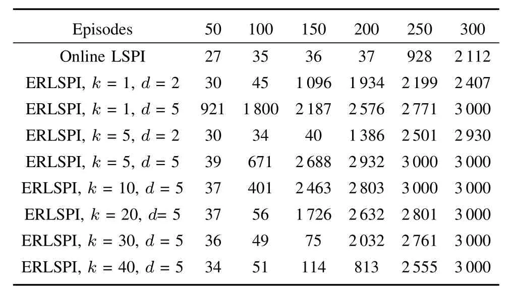
TABLE II THE BALANCING STEPSOFONLINE LSPIAND ERLSPI WITH LSTD-Q UNDER DIFFERENT PARAMETERS

Fig.3. The performance of online LSPIand ERLSPIw ith LSPE-Q under different parameters.

Table III shows the balancing steps of online LSPI and ERLSPIw ith LSPE-Q under different parameters in the fi rstp(p=50,100,150,200,250,300)episodes.Data in the table shows that,the balancing steps of online LSPIw ithin the fi rst150 episodes have been smaller than 50 steps,eventuallyreach 2112 steps w ithin the 300 episodes,while ind=5 ERLSPI,the balancing steps in dozens of episodes are up to severalhundred,and finally reach the 3000 balancing steps in 300 episodes.Therefore,reusing previous experience can significantly improve the performance of the algorithm and improve the convergence speed.In the case ofk＞5,whenkincreases,the computational costsbecome smallerand smaller,and so are the balancing steps,but they still reach the 3000 balancing steps in 300 episodes.

The performance comparison of ERLSPIand online LSPI,offl ine LSPI,Batch TD is shown in Fig.4,thebatch algorithms update the policy once every 5 episodes,the samples are reused 5 times,step size parameterα=0.005.The balancing steps of Batch TD in 300 episodes have been maintained w ithin dozens of steps,far lower than other least-squares methods,in which the least-squaresmethods add sample data to the matrix and make full use of the sample data.In online LSPI algorithm,the sample data is used only once,the initial performance is poor,but after about 230 episodes itgrows rapidly,while the initial performance of offl ine LSPI is better,because it reuses all the samples until the current policy is stable.Offl ine LSPI reuses samplesmost frequently,however,it requires samples collected in advance and cannot be supplemented w ith new and better online samples which lead to the slow grow th speed.ERLSPI algorithm collects samples online and reuses the sample data,which can ensure certain initialperformanceand quickly converge to theoptimal policy to achieve 3000 balancing steps.

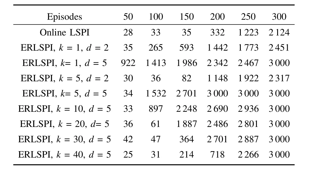
TABLE III THE BALANCING STEPSOFONLINE LSPIAND ERLSPIW ITH LSPE-Q UNDER DIFFERENT PARAMETERS

Define themean squared error(MSE)of policy parameterθas

whereθ∗is the optimal policy parameter,andNis the dimension ofθ.MSE indicates the distance between the current policy and the optimal policy.The smaller the value of MSE is,the higher the accuracy of the policy is.The MSE valuesof ERLSPIalgorithms and online LSPI,offl ine LSPI,Batch TD are shown in Fig.5.TheMSE of Batch TD algorithm is large,indicating the policy accuracy is unsatisfactory;online LSPI improves the policy accuracy obviously,but the grow th speed isslow;whileoffl ine LSPIimprovesvery fastin thebeginning,but it levels off after about 120 episodes and is unable to find the optimal policy in 300 episodes;ERLSPIalgorithms almost find the optimal policy after about 200 episodes and maintain high policy accuracy.Therefore,we can conclude that ERLSPIalgorithms can improve the policy accuracy w ith the same episodes,find the optimal policy more quickly,enhance the empirical utilization rate and accelerate the convergence speed.

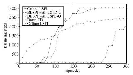
Fig.4. The balancing steps of different algorithms.

Fig.5. The MSE of different algorithms.

V.CONCLUSION

Traditionalonline least-squarespolicy iterationmethod uses the samples generated online only once which leads to the low empiricalutilization rate and slow convergence speed.We combine experience replay method w ith online least-squares policy iteration method and an ER least-squares policy iterationmethod isproposed.Themethod storessamplesgenerated online in the form of a tetrad(x,u,r,x′),and reuses these samples.In the process of experience reusing,although using the same samples in the form of tetrad,the policy parameter is updated w ith a quintuple(x,u,r,x′,h(x′)),and each policy is different in updating.As a result,samples can be used more than once to update the policy parameter to improve the empirical utilization rate.ERLSPIw ith LSTD-Q updates the policy parameter after processing a batch of samples,which hasmore stable performance;while the ERLSPIw ith LSPEQ updates the policy parameter after processing every sample and the result depends on the previous evaluation results.If a good initial value is assigned and the step size parameter is decreased gradually,it can also get good performance.Since the computation of the policy parameter needs to solve the matrix inversion which has high complexity and the large computational cost,the Sherman-Morrison formula is applied to the algorithm to elim inate thematrix inversion to reduce the time complexity and the computational cost.The experimental results of the inverted pendulum show that ERLSPImethod can reuse previous experience,improve the empirical utilization rate,and accelerate the convergence speed.Additionally,more repetitions bring aboutmore improvement,but requiring higher computational cost.Increasing the batch updating interval properly can also achieve a fine performancew ith smaller computational cost.Therefore,appropriate algorithm parametersshould be selected according to the specific circumstances.

When the state space is dividedmore finely,the dimension of radial basis functions becomes relatively larger.However,the least-squares method generally need high computational cost.How to reduce the computational costaswellas improve the computational efficiency and how to select the proper samples efficiently are very important which are our futureresearch work.In addition,transferring the work from the discrete action spaces to continuous action spaces is also our further study.

[1]Wiering M,van Otterlo M.Reinforcement learning:state-of-the-art.Adaptation,Learning,and Optim ization.Berlin,Heidelberg:Springer,2012.12−50

[2]Zhu Fei,Liu Quan,Fu Qi-M ing,Fu Yu-Chen.A leastsquare actor-critic approach for continuousaction space.JournalofComputerResearchand Development,2014,51(3):548−558(in Chinese)

[3]Liu De-Rong,Li Hong-Liang,Wang Ding.Data-based self-learning optimal control:research progress and prospects.Acta Automatica Sinica,2013,39(11):1858−1870(in Chinese)

[4]Zhu Mei-Qiang,Cheng Yu-Hu,LiM ing,Wang Xue-Song,Feng Huan-Ting.A hybrid transfer algorithm for reinforcement learning based on spectralmethod.Acta Automatica Sinica,2012,38(11):1765−1776(in Chinese)

[5]Chen Xin,WeiHai-Jun,Wu M in,CaoWei-Hua.Tracking learning based on Gaussian regression for multi-agent systems in continuous space.Acta Automatica Sinica,2013,39(12):2021−2031(in Chinese)

[6]Xu X,Zuo L,Huang Z H.Reinforcement learning algorithms w ith function approximation:recent advances and applications.Information Sciences,2014,261:1−31

[7]Bradtke S J,Barto A G.Linear least-squares algorithms for temporal difference learning.Recent Advances in Reinforcement Learning.New York:Springer,1996.33−57

[8]Escandell-Montero P,Mart´ınez-Mart´ınez JD,Soria-Olivas E,G´omez-Sanchis J.Least-squares temporal difference learning based on an extreme learning machine.Neurocomputing,2014,141:37−45

[9]Maei H R,Szepesv´ari C,Bhatnagar S,Sutton R S.Toward off-policy learning control w ith function approximation.In:Proceedings of the 27th International Conference on Machine Learning.Haifa:Omnipress,2010.719−726

[10]Tamar A,Castro D D,Mannor S.Temporal differencemethods for the variance of the reward to go.In:Proceedings of the 30th International Conference on Machine Learning(ICML-13).Atlanta,Georgia,2013.495−503

[11]Dann C,Neumann G,Peters J.Policy evaluation w ith temporal differences:a survey and comparison.The Journal ofMachine Learning Research,2014,15(1):809−883

[12]Lagoudakis M G,Parr R,Littman M L.Least-squaresmethods in reinforcement learning for control.M ethodsand ApplicationsofArtificial Intelligence.Berlin,Heidelberg:Springer,2002,2308:249−260

[13]LagoudakisM,Parr R.Leastsquarespolicy iteration.JournalofMachine Learning Research,2003,4,1107−1149

[14]Busoniu L,Babuska R,De Schutter B,Ernst D.Reinforcement Learning and Dynam ic Programm ing using Function Approximators.New York:CRC Press,2010.100−118

[15]Adam S,Busoniu L,Babuska R.Experience replay for real-time reinforcement learning control.IEEETransactionson Systems,Man,and Cybernetics,PartC:Applicationsand Reviews,2012,42(2):201−212

[16]Jung T,Polani D.Kernelizing LSPE(λ).In:Proceedings of the 2007 IEEE Symposium on Adaptive Dynamic Programming and Reinforcement Learning.Honolulu,HI:IEEE,2007.338−345

[17]Jung T,PolaniD.Least squares SVM for least squares TD learning.In:Proceedings of the 17th European Conference on Artificial Intelligence.Amsterdam:IOS Press,2006.499−503