Modeling and Verification of an Astronaut Handling Large-mass Payload

YANG Aiping, YANG Chunxin, *, and KE Peng

1 School of Aeronautics Science and Engineering, Beihang University, Beijing 100191, China

2 School of Transportation Science and Engineering, Beihang University, Beijing 100191, China

1 Introduction

Because of the high cost of astronaut extravehicular activity (EVA), it is necessary to conduct a detailed design beforehand and perform the training of astronauts’ tasks on the ground. Generally, such exercises are carried out at air bearing floors, neutral buoyancy tanks or aircraft flying parabolic trajectories. However, these facilities have some inner disadvantages such as friction on the air bearing floors, water damping in the neutral buoyancy tank, and narrow time span of the aircraft flying each parabola. It is necessary to simulate the astronauts’ task during EVAs.Therefore, the approach of computer simulation of the EVA tasks is especially essential There are many aspects related to research, such as the concept of advanced EVA systems[1,2], EVA worksites design[3], space-suited locomotion[4], astronaut reorientation[5]and so forth.

In the EVA tasks, the astronauts frequently need to handle the large-mass payload from one worksite to another.In order to make a good training project related to such a task, the basic kinematics and dynamics characteristics about the astronauts must be known. NEWMAN and SCHAFFNER[6,7]of the Massachusettes Institute of Technology performed the computer simulation involving the manipulation of a large-mass payload based on inverse kinematics and Kane method supported by NASA. Their research revealed a process of simulating astronaut task via the computational multi-body dynamics, although the mechanical effects of a space suit are not accounted for.YANG, et al[8,9], studied the suited astronaut movement based on the Kane method; their contribution is to add the mass properties of each segment of extra vehicle mobility unit (EMU) to the corresponding segment of the astronaut model.

The goal of this study is to solve the joint angles and joint torques of the astronauts handling a large-mass payload based on inverse kinematics and inverse recursive dynamics, and also to validate the results with the ADAMSTMvirtual model. The differences between this study and the results from other studies are that the torque of each joint in time interval can be obtained under the constraints of the least velocity and acceleration of each joint, and that the results calculated can be verified by the ADAMSTMvirtual model. The approach to calculating joint torques of the specific astronaut motion in detail is presented via minimizing joint velocities and accelerations.In addition, the process of verifying the above results by establishing the ADAMSTMvirtual model is illustrated.

The remainder of this paper is arranged as follows:Section 2 describes the modeling methods of the EVA task,and gives the flow chart of solving joint angles and torques.The joint motion data which include joint angles, joint velocities, joint accelerations and joint torques in time domain are calculated and discussed. Subsequently, the simulation verification is performed by the ADAMSTMvirtual model in section 3. Conclusions are drawn in section 4.

2 Modeling Methods for the Astronaut EVA Task and Process of Solving Joint Motion

The modeling methods consist of four steps: task description, geometric model, forward and inverse kinematics, and inverse recursive dynamics. Then, the flow chart of solving joint angle and torque is given.

2.1 Task description

An astronaut of fixed feet to handle a large-mass payload[10]is taken as an example of the EVA task. The payload is Spartan astronomy payload in STS-63 flying tasks[6], 1 201.4 kg in mass and 1.344 m×1.241 m×1.309 m in dimension. The astronaut motion model is to manipulate the payload with his arms around a circle trajectory counterclockwise motion in the human body sagittal plane. The radius of the circle is 0.075 m.

2.2 Geometric model

A simplified model of an astronaut based on Hanavan’s fifteen body finite-segment model of the human body is shown in Fig. 1.

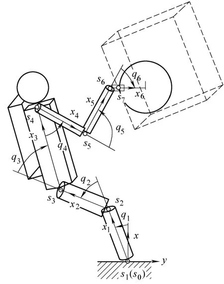
Fig. 1. Model of an astronaut handling large-mass payload

This model consists of upper arm, forearm, hand, trunk,upper leg, lower leg and foot, which are connected respectively with revolute joints. The upper arm, forearm,upper leg, and lower leg are viewed as frustums of cones,the trunk is an elliptical cylinder, and the hand is a thin cube. Payload is added to the center of mass of the hand.Thus, the model is regarded as a planar movement of a multi-body system which includes seven segments with six revolute joints in the human body sagittal plane.

The inertial frame shown in Fig. 1 is set up at the ankle joint, where the x coordinate is horizontal right, and the y coordinate is vertical upwards. The end motion equations can be obtained as follows:

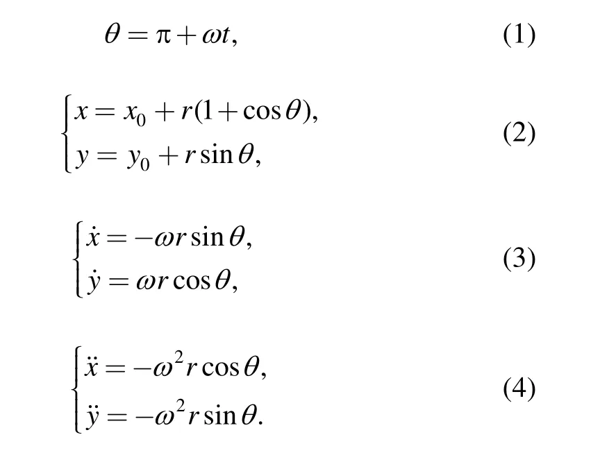
Where θ is the angle of the center of mass of the hand,ω is the angular velocity of circle trajectory, t is time,r is radius of circle, and x and y are the coordinates of the center of mass of the hand in the inertial frame, respectively.and y0are the initial positions of x and y,andare the velocities of the center of mass of the hand,anddenote the accelerations of the center of mass of the hand.

2.3 Forward kinematics

The forward kinematics method is used to solve the kinematics parameters of the center of mass of the hand by using joint space variations in the following steps.

First, joint angleiq(i = 1, 2, …, 6) is defined as generalized coordinates of the multi-body system, and inertial frame and local joint frames are set up as shown in Fig. 1. s0represents the inertial frame which is fixed on foot,is(i = 1, 2, …, 6) denotes the local joint i frame, xiis the horizontal axis of joint i which the orientation is from joint i to joint i +1. Each joint rotation axis is vertical to paper outwards.

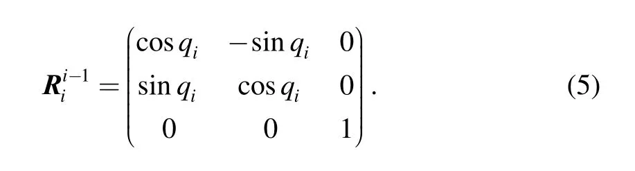
Secondly, the transformation matrixabout local joint i frame relative to local joint i–1 frame is described:

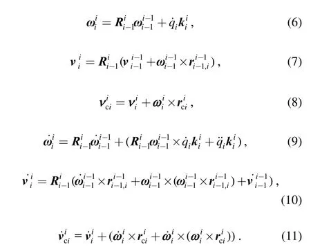
Finally, on the basis of the kinematics of multi-body mechanics[13], the local joint kinematics parameters in the local joint frame can be calculated. Angular velocity, linear velocity, angular acceleration, and linear acceleration at the local joint i frame can be obtained from Eqs. (6), (7), (9),and (10). The velocity and acceleration of the mass center of link i can be achieved from Eqs. (8) and (11):

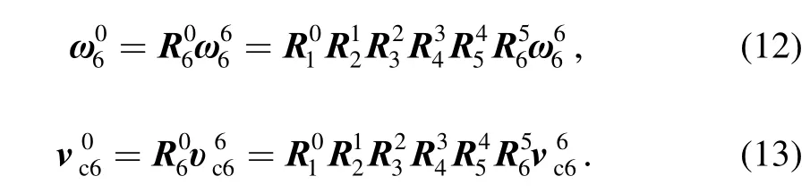
Therefore, the series transformation matrix can be obtained with Eq. (5). For each joint, we can obtain the corresponding transformation matrix expression. The linear velocity and angular velocity of the center of mass of the hand at the inertial frame can be obtained from Eqs. (13)and (12):

In Eq. (13), we can obtain matrix J in Eq. (14) by partially differentiating to joint speeds.

2.4 Inverse kinematics

The inverse kinematics is used to solve joint space kinematics parameters with known operation space motion trajectory. For serial chain and tree-structured system[14], a relation expression with the velocities in operation space and the velocities in joint space is described as

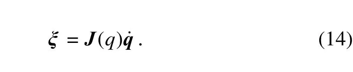
In this plane model, ξ ∈R2is known by Eq. (3), andcan be solved by partial differentiating Eq.(13), and then we can determinein Eq. (14); thus,q andcan be obtained by integration and derivation torespectively.

To obtain the determinate q, the generalandcan be computed by Eqs. (15) and (16):

Where+

J denotes the pseudo inverse of J(q) ,φ denotes an arbitrary vector inspace. Here we attain specificandwhen φ=0 ; thus,and˙ are the least.

2.5 Inverse recursive dynamics

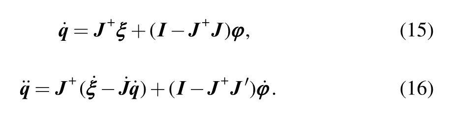
Inverse recursive dynamics for the above articulated figure model, which is considered as serial multi-link tree-structure system can be described as follows[7]:

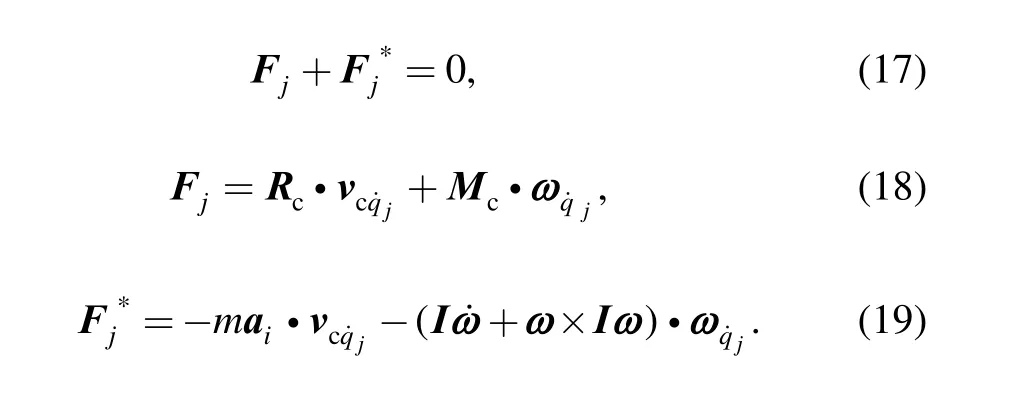
Where Fjand F*jare respectively the generalized force and initial force of the mass center of rigid body j.cR and Mcrepresent the force and torque acted on the mass center of rigid body j, respectively. ν c q˙j is the partial linear velocity forwhich is solved by partial differentiating Eq. (8) , and ωq˙jis the partial angular velocity, which is achieved by partial differentiating Eq. (6).m is the mass of the rigid body. aiis the acceleration of the mass center of the rigid body. I is the moment of inertia for the mass center of rigid body.

By Eq. (17), the following equation can be easily obtained for the multi-rigid body system:

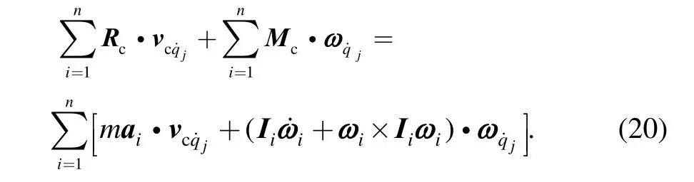
Where n is the number of the links of multi-rigid body system.

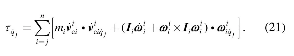
By analyzing the forces acted on the links, the joint torque for joint i can be calculated by using Eq. (21), thus,all joint torques can be solved with these recursive formulations, and the results are given in the condition of the least velocity and acceleration of each joint as explained in Eqs. (15) and (16):

2.6 Flow chart of solving joint angle and torque

The flow chart given in Fig. 2 illustrates the solution process of solving joint angle and torque.

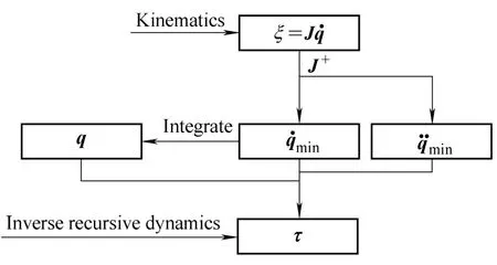
Fig. 2. Solution process of solving joint angle and torque

The system studied in this paper has six degrees of freedom. The center of mass of the hand has three degrees of freedom, which include two planar displacements and one rotation to z axis. On the basis of the above analysis,it can be concluded that this system has three redundancies.Therefore, the joint speeds of Eq. (14) in this system have multi-solutions. In order to obtain the joint determinate speed solution,can be achieved based on the cost of minimizing the Euclidean module in Eq. (14). Each joint angle q can be obtained by integrating these velocities over time.can also be calculated by the same way as solving. First, for differentiating Eq. (14) over time, we can determine the expression including ofvariation.Second,can be achieved by minimizing the Euclidean module on the expression including ofvariation.

3 Calculation of Joint Angles and Torques and Discussion

The motion studied in this paper is a planar movement of a multi-body system, which includes seven segments with six revolute joints in the human body sagittal plane as shown in Fig. 1. The mass center of an astronaut’s hand is assumed as a circular trajectory using counterclockwise arm motions; one period movement is finished within 20 s.

The respective mass properties of each segment of the EMU can be added to the corresponding human body segment according to the geometrical size of the human body and the mass properties[8]. Thus the moment of inertia about the mass center of each segment can be calculated.The geometric size and mass properties of the model in this paper are shown in Table 1[8,11]. As shown in Table 2, the limits of the EMU joint movement are given[12].

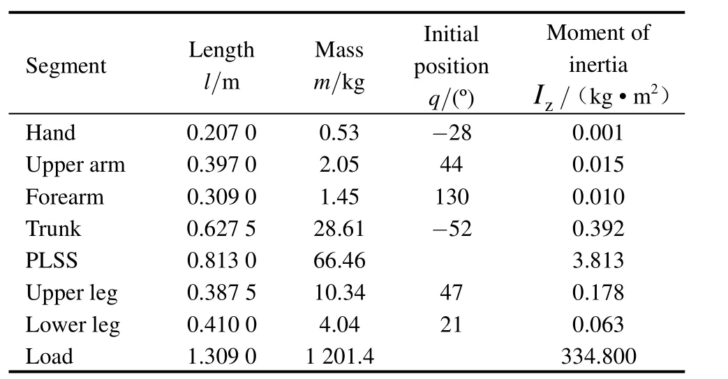
Table 1. Geometric size and mass properties of the model

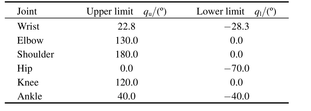
Table 2. Limit of the EMU joint movement

The variation of each joint angle with movement time calculated using the simplified model is shown in Fig. 3.The peak values of all joint angles are within the EMU joint restrictions.

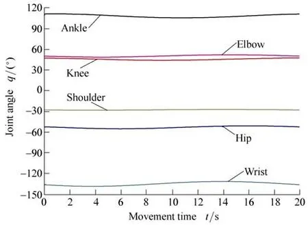
Fig. 3. Joints angle plots

The variation of the six joint angular velocities and accelerations with movement time are shown in Fig. 4 and Fig. 5, respectively. The results show a smooth changing of the six joint velocities and accelerations within one period.Based on the above computing method, it can be concluded that the joint angular velocities and accelerations calculated in this model are the least.

Fig. 6 indicates the torque curves of six joints during one period. All curves show smooth cosinusoidal curves. The limits of each joint torque both calculated in this paper and Refs. [11-12] are shown in Table 3. For the four torques,except for the hip and ankle torques, the results are found in Refs. [11-12] for comparison which indicates that the four joints’ torques are within the limits obtained by the experimentation in Refs. [11-12].

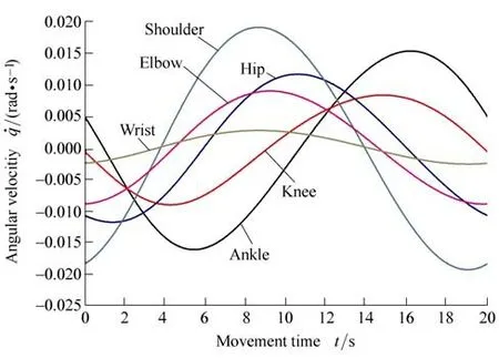
Fig. 4. Joints angular velocity plots

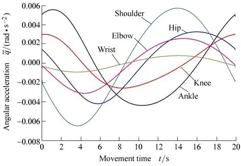
Fig. 5. Joints angular acceleration plots

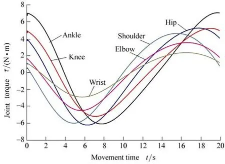
Fig. 6. Joints torque plots

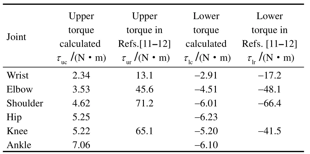
Table 3. Limits of each joint torque both result calculated in this paper and Refs. [11–12]

4 Simulation Verification

In this section, the simulation using the ADAMSTMmodel is used to verify the calculated results. The ADAMSTMsoftware applies the Lagrange method of multi-body dynamics for setting up dynamical equations[15,16].

4.1 Virtual model

The astronaut simplified model of Fig. 1 was built in the ADAMSTMsoftware. The geometric size and mass properties of the model is defined according to Table 1.

4.2 Flow chart of verification

Fig. 7 shows the flow chart of verification. Four steps were used to verify the results calculated in this paper. The first step was to build a virtual model with the ADAMSTMsoftware. The next step was to perform motion simulation via adding rotational joint motion to six joints of virtual model. Here, joint kinematical parameters such as the joint angles calculated were used to rotate the joint motion. The third step was to create the trace the center of mass of the hand and compare with the known circle of the center of mass of the hand. If the two circles are essentially overlapped, it indicates that joint kinematical parameters calculated in this paper are exact. The fourth step was to measure the kinematical and dynamical parameters of virtual model joints in order to compare with the corresponding data calculated in this paper.

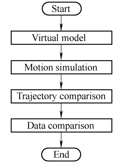
Fig. 7. Flow chart of verification

4.3 Trajectory verification

The joint kinematical data calculated in the paper is applied to drive the rotational joint of the virtual model. In addition, the trace of the central mass of hand is obtained and denoted with the blue circle in Fig. 8. The red circle is the known trace of the center of mass of the hand. Since the two circles are coincident, the joint kinematical data can be judged exact. That is to say, joint kinematics data calculated including joint angle, velocity, and acceleration are exact.

4.4 Data verification

The joint kinematical and dynamical parameters during one simulation period can be measured and compared with the corresponding data calculated in this paper.

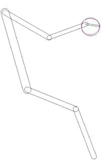
Fig. 8. Trajectories of the center of mass of the hand (red circle for virtual model,blue one for known trajectory)

Fig. 9 and Fig. 10 show six joint angular acceleration curves and six joint angular velocity curves, respectively. It is shown that the six measuring curves with star-shaped figures obtained from proposed method are coincident with the six calculated curves with solid lines for the ADAMSTM.Therefore, the joint velocities and acceleration calculated in this paper are exact.

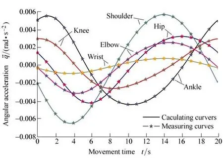
Fig. 9. Joints angular acceleration comparison

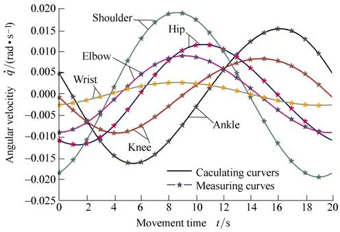
Fig. 10. Joints angular velocity comparison

Fig. 11 displays six joint angle curves during one period.By comparing six measuring curves denoted with star-shaped figures to six calculated curves plotted with solid lines, it is seen that two curves of each joint are coincident. Therefore, the joint angles calculated in the paper are exact.

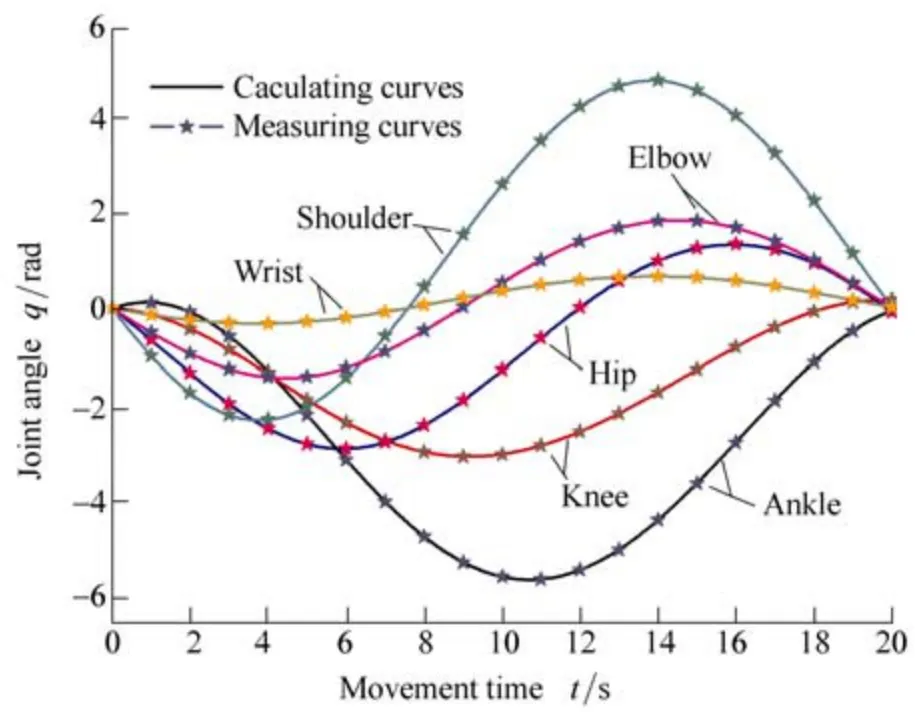
Fig. 11. Joints angle comparison

The joint angle, velocity, and acceleration data series calculated in this paper are compared with ADAMSTMmeasuring one. As a result, two data series of each joint from different methods are identically distributed.Therefore, it is revealed that the kinematical data calculated are exact.

Fig. 12 illustrates six joint torque curves. Comparing the six measuring curves with star-shaped figures to the six calculated curves with solid lines proves that two curves of each joint are essentially coincident. However, there are some departures between the measuring curves and the calculated one, because the torque of each joint has a variation with its joint angle; the velocity and acceleration according to Eq. (21), also the angle and acceleration of each joint are obtained by taking a differentiation of the joint velocity

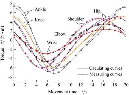
Fig. 12. Joints torque comparison

5 Conclusions

(1) A simplified model of an astronaut was built, and the astronaut motion was conceived as a planer movement of a multi-body system, which included seven segments with six revolute joints in the human body sagittal plane.

(2) The inverse kinematics method can be employed to calculate joint angles, joint velocities, and joint accelerations in time domain. Furthermore, joint torques can be solved by using the inverse recursive dynamics. The virtual model can be constructed with the ADAMSTMsoftware to verify the calculated results.

(3) The simulation verification indicated that the computing methods presented, which consists of the forward and inverse kinematics and the inverse recursive dynamics,were feasible and the ADAMSTMvirtual model can be used as an efficient and effective tool to verify the results calculated for the basic kinematics and dynamics characteristics about the astronaut's tasks.

[1] DAVID C, DIANE M,MICHELLE M, et al. Concepts for advanced extravehicular activity systems to support NASA’s vision for space exploration[C]// Proceedings of the44th AIAA Aerospace Sciences Meeting and Exhibit, Reno, Nevada, 2006: 348–356.

[2] JORDAN N C, SALEH J H, NEWMAN D J. The case for an integrated systems approach to extravehicular activity[C]//Proceedings of the 1st Space Exploration Conference: Continuing the Voyage of Discovery. Orlando, Florida, 2005: 2 782–2 786.

[3] COAN D A, KAGEY J L. Developing and verifying requirements for extravehicular activity (EVA) worksites[C]// Proceedings of the space 2005, Long Beach, California, 2005: 6 629–6 643.

[4] CARR C E, NEWMAN D J. Characterization of a lower-body exoskeleton for simulation of space-suited locomotion[J]. Acta Astronautica, 2008, 62: 308–323.

[5] STIRLING L, WILLCOX K, NEWMAN D J. Development of a computational model for astronaut reorientation [J/OL]. Journal of Biomechanics, 2010-05-17[2010-05-28]. http://www.jbiomech.com/article/S0021-9290(10)00244-7/abstract.

[6] NEWMAN D J, SCHAFFNER G. Computational dynamic analysis of extravehicular activity (EVA): large mass handling[J]. Journal of Spacecraft and Rockets, 1998, 2(35): 225–227.

[7] NEWMAN D J, SCHAFFNER G. Dynamic analysis of astronaut motions in microgravity: applications for extravehicular activity(EVA)[R]. MIT: NASA-CR-199668, 1996.

[8] YANG Feng, YUAN Xiugan, LI Yinxia. Computational simulation of extravehicular activity[J]. Journal of System Simulation, 2003,2(15): 216–225. (in Chinese).

[9] YANG Feng, YUAN Xiugan. Application of Kane’s method in simulating extra vehicular activity[J]. Chinese Journal of Applied Mechanics, 2004, 21(2): 151–154. (in Chinese).

[10] RICCIO G E, VERNON MCDNALD P, PETERS B T, et al.Understanding skill in EVA mass handling volume I: theoretical &operational foundations[R]. NASA TP-3684, 1997.

[11] MORGAN D, WILMINGTON R P, PANDYA A K, et al.Comparison of extravehicular mobility unit(EMU) and unsuited isolated joint strength measurements[R]. NASA TP-3613, 1996.

[12] Man Systems Integration Standards. NASA STD-3000[S]. Houston:Johnson Space Center, 1995, 1(B): 585–642.

[13] MA Xiangfeng. The robot mechanisms[M]. Beijing: China Machine Press, 1991. (in Chinese).

[14] XIONG Youlun. The Robotics[M]. Beijing: China Machine Press,1993. (in Chinese).

[15] ZHENG Kai, WU Xiren, CHEN Loumin, et al. ADAMS 2005 advanced application examples for mechanical design[M]. Beijing:China Machine Press, 2006. (in Chinese).

[16] LIU Ning, LI Junfeng, FENG Qingyi, et al. Underwater human model simulation based on ADAMS[J]. Journal of System Simulation, 2007, 19(2): 240–243. (in Chinese).