New Method to Measure the Fill Level of the Ball Mill I—Theoretical Analysis and DEM Simulation

HUANG Peng, JIA Minping, and ZHONG Binglin

School of Mechanical Engineering, Southeast University, Nanjing 211189, China

1 Introduction

The ball mill pulverizing system has the advantages of good adaptability for different types of coal and easy maintenance, and has been applied widely for comminuting and drying coal in coal-fired power plant. At the same time this system consumes high energy that makes up about 20 percent of all electricity consumption of power plant. So making the mill operation safely and having high efficiency are important goals for power plant. Because the ball mill pulverizing system is non-linearity, long time delay and time-varying, the fill level of coal powder can not be measured accurately, which leads the mill to be operated usually under the very uneconomical condition to prevent the coal blockage. Furthermore it is difficult for the automatic control system to accomplish the steady operation of the mill. Therefore the exact measurement of the fill level is a key and basic factor for realizing automatic, reliable and efficient operation of the mill system.

Many methods have been applied for measuring the fill level. One of traditional methods was that the fill level can be measured as a function of the differential pressure between the inlet and the outlet of the mill. As the fill level increases, more coal powder is exposed to the air flow through the mill, air drag forces are high, and the differential pressure increases. The same relationship concerns the opposite condition, as the fill level decreases.ZHANG studied the fill level by measuring the power consumption of the mill motor[1]. KOLACZ put forward a method to measure the fill level by using a strain transducer[2]. The transducer was installed at the middle of the mill shell. When the transducer was in the top position of the mill shell, compression was measured by the transducer. When the transducer reached the bottom of the mill shell along with the rotation of the mill, tension was measured by the transducer. By taking the difference between the readings corresponding to compression and tension, it was possible to calculate the total strain variations that are directly proportional to the fill level.Recently the measurement and control of the fill level in the mill have also been accomplished by analyzing the acoustic signals of the mill[3–5]. Together with the increment of the fill level, the acoustic signal presents a decreasing trend, and vice versa. Since the vibration strength of the mill shell and the bearing housings can reflect the information of the fill level, vibration methods have recently been carried out to develop techniques for monitoring the fill level. Among these vibration methods,the fill level can be measured through extracting some characteristic values from the vibration signals of the bearing housings, such as amplitude, energy, power and root mean square (RMS)[6–8].

To sum up above works, some factors and variables, such as the steel ball load, coal property and the disturbance of other noise near the mill can affect the main variables corrective to the fill level and the measured result. For example, the amplitude of acoustic and vibration signal of the mill has a greater difference under the same fill level condition by the variation of the ball load and the water content of coal, and the power of the mill is also influenced seriously by the change of steel ball load. The main goal of this paper is to put up a new method for measuring the fill level through studying the relation between the fill level and the position of the maximum vibration point on the mill shell. In this paper, this relation is researched by two approaches. One is theoretical analysis method, and another is the DEM simulation method. At the same tine the results of the theoretical calculation and the DEM simulation are compared and discussed. Finally, in the second part (II) of this research, the vibration signals that are directly collected off of the mill shell under various experiment conditions are analyzed to verify the results and conclusions of the first part (I) of this research.

2 Theoretical Calculation

Compared with steel balls in other layers, the steel balls in the outmost layer have the greatest impulse and kinetic energy in the course of falling, and the maximum vibration point on the mill shell is generated by the falling impact of steel balls in this layer. The positions of the outmost layer steel balls can be seen in Fig. 1.

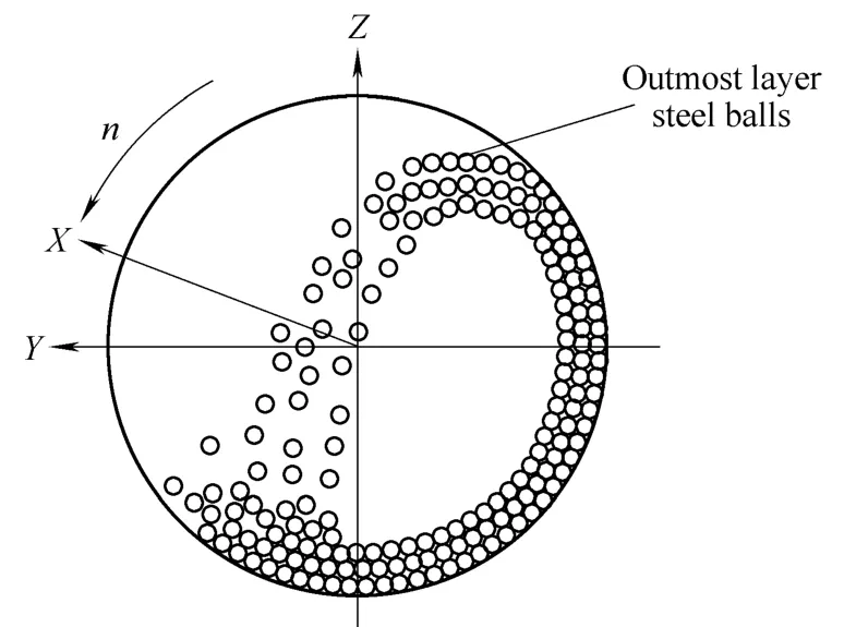
Fig. 1. Schematic diagram of motion of the steel balls in many layers in the mill

When the outmost layer steel ball impacts directly on the mill wall, the collision point is the maximum vibration point of the mill shell. When the steel ball in the outmost layer impacts on coal particles, the impact energy is delivered to the mill shell, which also leads to a maximum vibration point on the mill shell. In this research, the relationship between the fill level and the position of the maximum vibration point of the mill shell is tried to study on the first time. If this relationship can show certain regularity, the fill level can be studied by this point.

In this research, the fill level is defined as follows:

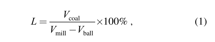
where Vmillis the effective volume of the mill, m3; Vballis the accumulated volume of the steel balls inside the mill,m3; Vcoalis the accumulation volume of the coal particles and powder inside the mill, m3.

The position of the maximum vibration point of the mill shell is calculated theoretically under two assumptions described as follows.

(1) During the work process of the mill, except for a steel ball in the outmost layer, as shown in Fig. 2, the coal particles and other steel balls are accumulated at the bottom of the roller at static state. In Fig. 2, the length of line CH denotes the accumulated height of the coal particles and steel balls in the mill, and the line AE represents the accumulation surface.

(2) In Fig. 2, there is no displacement in the x direction for the movement trajectory of the ball in the outmost layer,and x coordinate of this ball is always equal to zero.

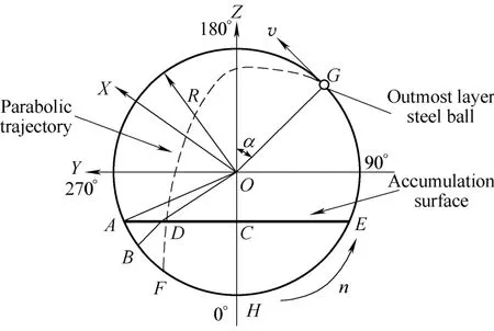
Fig. 2. Schematic diagram of motion trajectory of the outmost steel ball in the mill

When the ball reaches the detachment point G, as shown in Fig. 2, this ball begins a parabolic movement. The intersection point (collision point) between this parabolic trajectory and accumulation surface is point D (0, a, b). In the falling course, when the steel balls impacts on the coal particles, the part of impact energy of steel balls is absorbed by coal particles to realize the grinding and comminuting of coal, and another part of impact energy is delivered from the collision point to the mill shell and causes the vibration of the shell. So the position of the maximum vibration point on the mill shell is at a minimum distance from the collision point, and point B (0, y, z) (see Fig. 2) denotes the maximum vibration point. Here the minimum distance is obtained with a restrictive condition,which is expressed by

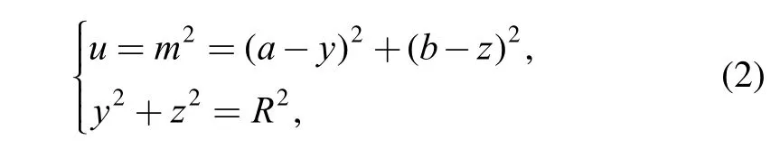
where m is the distance between point B and point D. In Eq.(2), the minimum value of u is needed, and the following formula can be obtained by the restrictive condition:

Then parameter u can be calculated as follows:

Eq. (4) taking the derivative of y at both its ends can be determined by

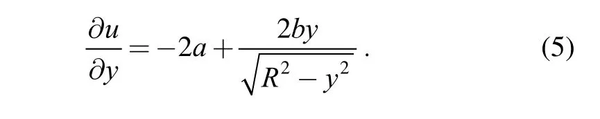
Zero value is given the left end of Eq. (5), and y coordinate of point B can be obtained by

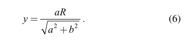
And then z coordinate of point B can also be obtained by

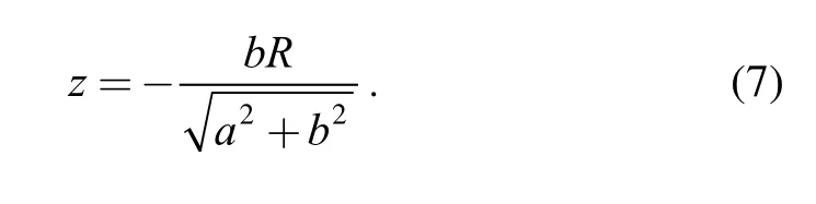
In Fig. 2, point D is the intersection point of the parabolic trajectory GF and the accumulation surface AE,and this parabolic trajectory and accumulation surface can be described by the following equations:

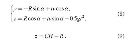
The coordinates of point D can be gained by the Eqs. (8)and (9). In the on-site tests, a 3.5 m diameter by 6.0 m long industrial tubular ball mill was operated at 17.57 r/min(77% of critical speed), and this mill filled by 38 t steel balls with diameter from 0.04 m to 0.06 m. When the mill is operated with 15% fill level, the coordinates of point D(0, 0.35 m, −0.65 m) can be calculated, and then the coordinates of point B (0, 0.83 m, −1.54 m) can be obtained easily by means of Eqs. (6) and (7). At the same time the value of ∠B OC(see Fig. 2) can be calculated by the coordinates of point B and is equal to 28.3º. In Fig. 2,the position of point B locates at 331.7º on the mill shell,and this angle (331.7º) represents the angular position of the maximum vibration point on the mill shell. This angular position is denoted by the parameter θ in this paper. By a similar principle, the coordinates of point D and point B,and the angular positions of point B for 0%, 5% and 10%fill level cases can be calculated, and the calculated results are shown in Table 1.

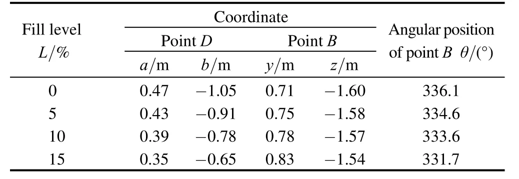
Table 1. Coordinates of points D and B, the angular positions of point B for four levels of fill level

As evident from Fig. 3, the angular position of the maximum vibration point on the mill shell decreases with the increase in the fill level. However this result is obtained under the ideal conditions. Many factors, such as the collision between ball and ball or the mill wall, the motion of coal and steel balls, have not been considered, so this conclusion needs to be verified further by other approaches.Once this conclusion can be validated, which can provide a new theory and method for measuring the fill level. In the next content, the 3-dimensional DEM simulations are performed to predict the load behaviour, motion trajectory of the outmost layer steel balls and the mill power draw.And the DEM simulated results will be compared and discussed with the results of the theoretical calculation.

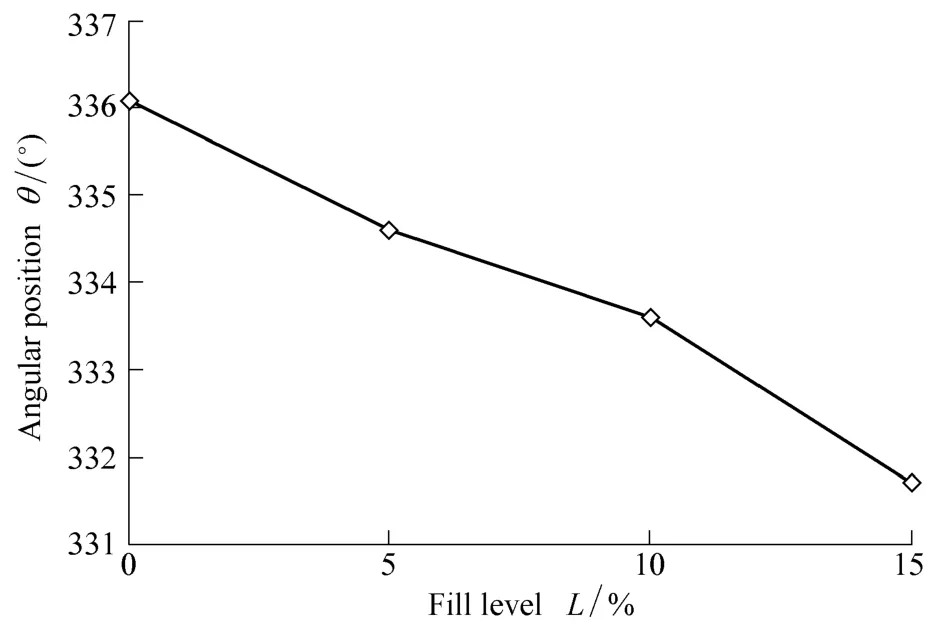
Fig. 3. Vibration in the angular position of point B (the maximum vibration point) on the mill shell with the fill level

3 3D DEM Simulation of Charge Motion of the Mill

3.1 Discrete element method

The DEM was originated in 1971 by CUNDALL for the analysis of rock-mechanics problems and then was applied to model the behavior of soil particles under dynamic loading conditions by CUDALL and STRACK[9]. The DEM refers to a numerical scheme that allows finite rotations and displacement of rigid bodies, where complete loss of contacts and formation of new contacts between bodies take place as the calculation cycle progresses. And the DEM is basically a numerical method by which the dynamic behaviour of the particles or bodies in a physical system is simulated with the particles being treated as distinct but interacting element. According to the advantage of the DEM and the work mechanism of the mill, the DEM suits to resolve the problem of the mill. Since the DEM was firstly used in the milling by MISHRA and RAJAMANI[10],there were some successful applications of the DEM in solving various tumbling mill problems[11–14]. The theory and principle of DEM can be acquired in detail from Refs.[15-17], it is only introduced briefly in this paper. In the DEM model, the steel balls and coal particles are simulated as the smooth round sphere and contacts by them with other balls and walls are considered to be distinct single-point contacts. The ball-to-ball and ball-to-wall collisions are modeled by the DEM with a linear spring and dashpot. The spring provides the repulsive force, and the dashpot dissipates a portion of the relative kinetic energy. In the following, the ball-ball collision model is illustrated to introduce the motion and force of the ball. The ball-wall collision is simulated in a similar manner. Fig. 4 is a schematic diagram of ball A and ball B in collision.

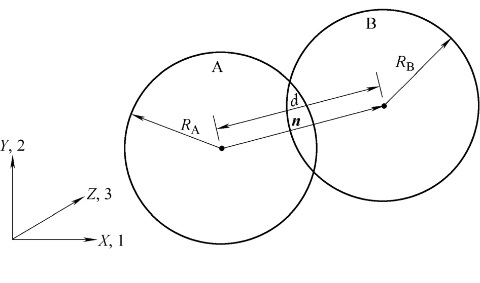
Fig. 4. Schematic diagram of ball A to ball B in collision

For the ball-ball contact, the unit normal vector, n, from the center of ball A to that of ball B that defines the contact plane, is given by

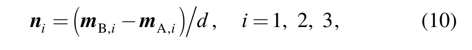
where mA,iand mB,iare the position vectors of the centers of balls A and B, and d is the distance between the ball centers:

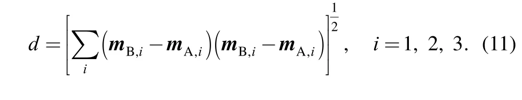
The contact velocity vi, which is defined as the velocity of ball B relative to ball A at the contact point, is given by

The normal and shear components of viare

The contact force vector Fiwhich represents the action of ball A on ball B can be resolved into normal and shear components with respect to the contact plane as

where Fn,iand Fs,idenote the normal and shear component vectors, respectively.

3.2 3D DEM simulation and verification

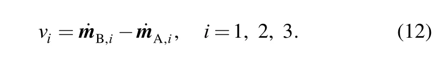
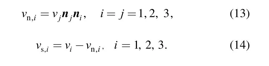
The speed, size of the mill, steel ball load and radii of steel balls that are the same with those of the experimental mill are simulated by the DEM. The coal particles are modeled as sphere, and the radius of coal ball is 0.01 m. As shown in Fig. 5, the charge motions of the mill for four levels of fill level (0%, 5%, 0% and 15%) are simulated,respectively.

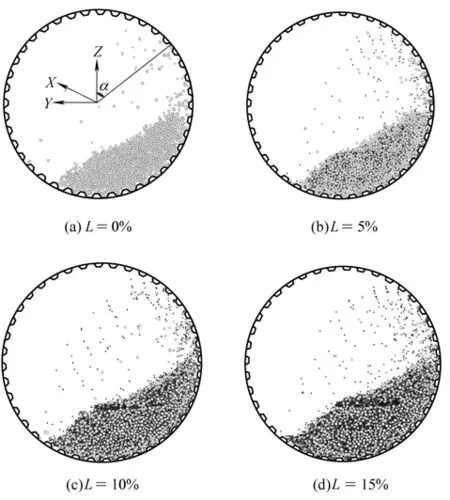
Fig. 5. Simulated charge motion of the ball mill by the DEM

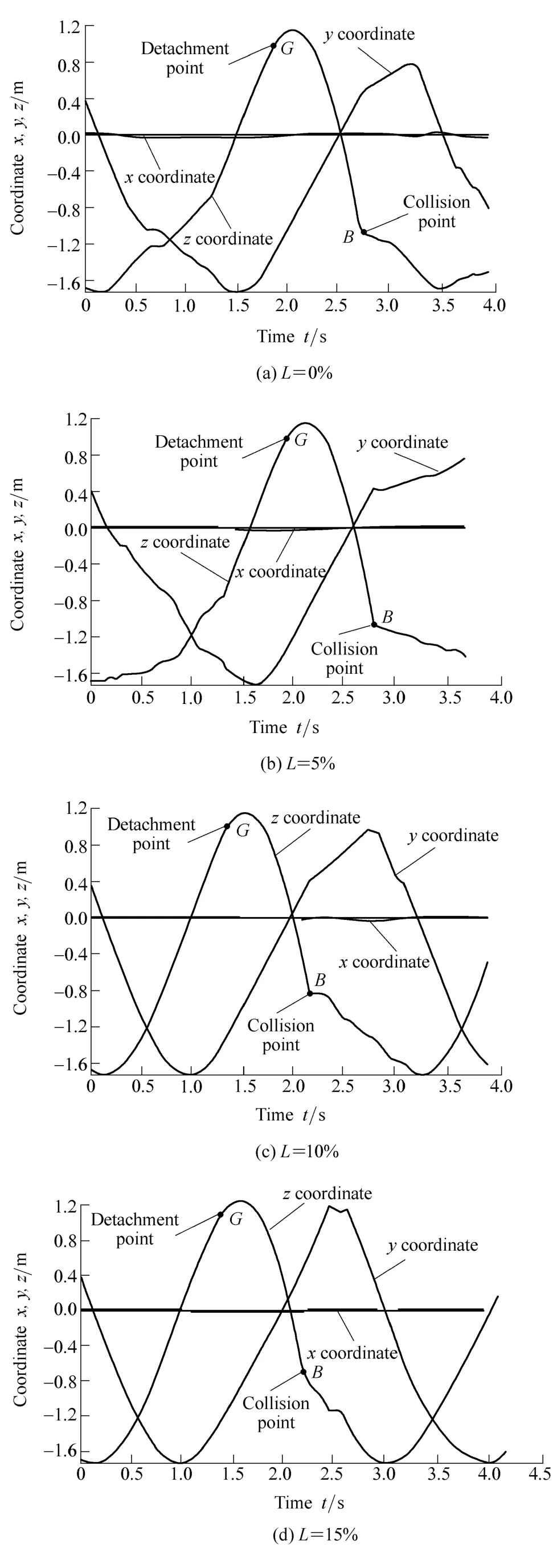
Fig. 6. Variation of coordinates of the ball C with time during 4 s in the DEM simulation

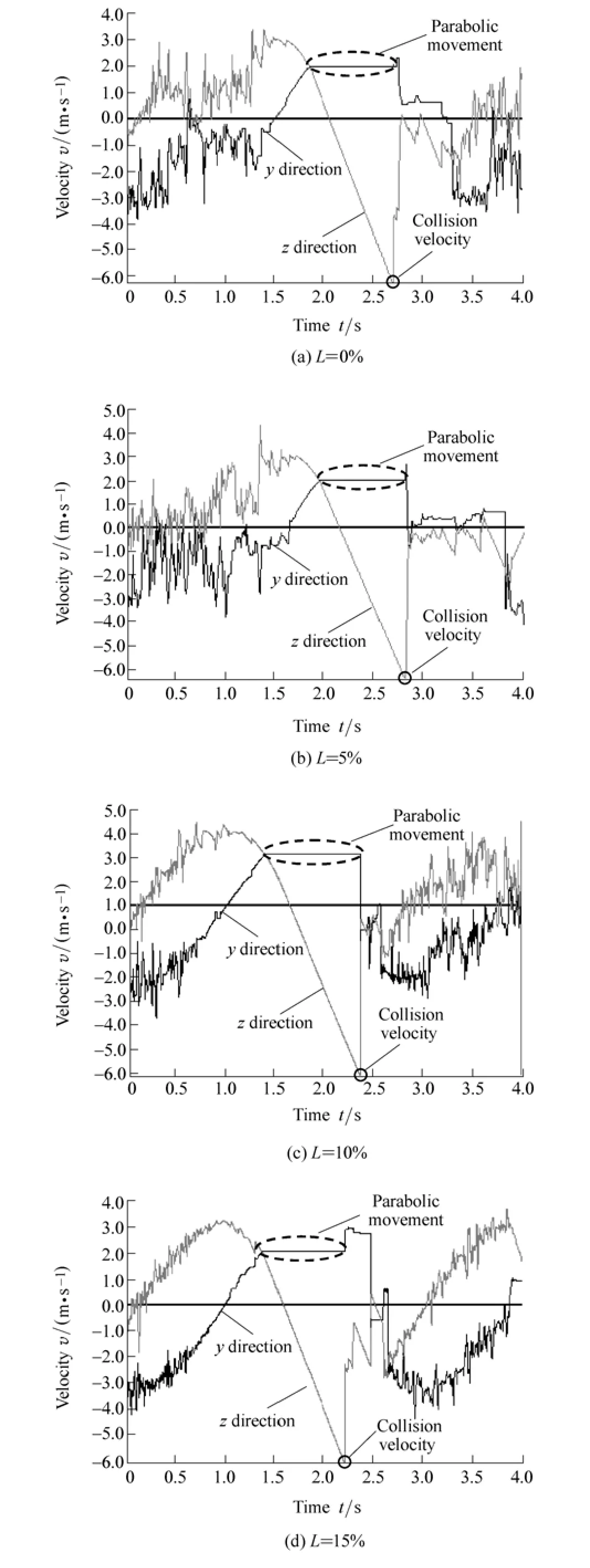
Fig. 7. Variation of velocities of ball C with time during 4 s in the DEM simulation

In this study, two methods are used to verify the simulated results. One is to compare the simulated and theoretical trajectories of the steel balls, and another is to compare the simulated and experimental power draft values of the mill. Because the charge motion of the experimental industrial mill can not be photographed by the camera, the simulated charge motion was only compared with the theoretical charge motion of the test mill in this research.The cataracting trajectories of the outer balls and cascading trajectories of the inner balls, as shown in Fig. 5, agree closely with the theoretic trajectories. In the DEM simulation, the positions and velocities of the steel ball C in the outmost layer were monitored. Fig. 6 shows the changes of positions (x, y and z coordinate) of the ball C with respect to time for four levels of fill level (0%, 5%,10% and 15%), respectively. And Fig. 7 shows the changes of velocities (y and z direction) of the ball C with respect to time for four levels of fill level (0%, 5%, 10% and 15%),respectively.

In Fig. 6, when the time is equal to zero, ball C (0, 0.36m,−1.71m) locates at the outmost layer of the steel balls in the mill and clings to the mill wall. When the mill begins to rotate, ball C runs circular movement firstly, which can be reflected by the changes of y and z coordinates of ball C in Fig. 6. Once ball C passes across the detachment point G,ball C starts to do parabolic movement, which can be demonstrated by the constant velocity process in y direction in Fig. 7. And the processes of parabolic movement are tagged by four ellipses in Fig. 7(a), 7(b), 7(c) and 7(d),respectively. When ball C in y direction begins to do uniform motion, this ball locates at the detachment point,and the coordinates of this point can be gained from Fig. 6.Table 2 shows a comparison of theoretic and simulated values of positions and velocities of detachment point for ball C. An exact match between the simulated and theoretic values can be obtained from Table 2, which can clarify the positions of the toe and shoulder of the ball charge are also closely matched.

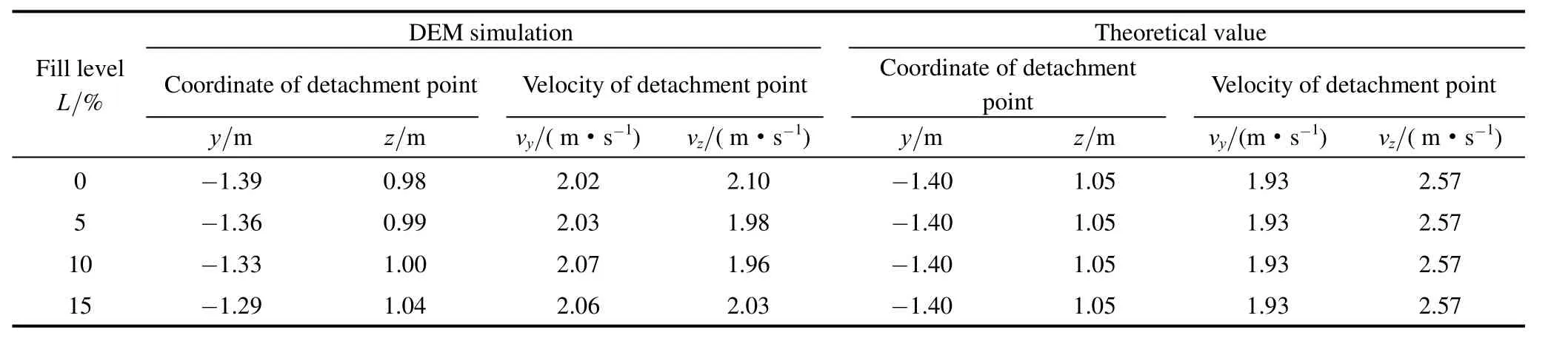
Table 2. Comparison of theoretic and simulated values of positions and velocities of the detachment point for ball C

Since the laws of motion imply that velocity,acceleration, force, power and energy are related,predicting power successfully is tantamount to predicting the other quantities correctly as well[17]. At the same time the power of the mill is obtained easily in the experiment.So the comparison between the simulated and experimental power draft of the mill is a good way to verify the DEM simulation. A comparison of the simulated and experimental power draft values of the mill is shown in Table 3. On comparison, it can be seen clearly that the simulated and experimental power values matches very closely. So the DEM simulation of the mill is reliable.

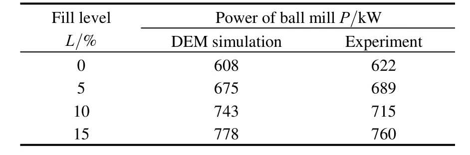
Table 3. Comparison of simulated and experimental mill power values

3.3 Analysis of motion trajectory of the outmost layer steel ball

During the period of parabolic movement, ball C does uniform motion in y direction, and does free fall motion in z direction, which can be demonstrated by the changes of velocities in y and z directions in Fig. 7. When the velocity of ball C in z direction reaches at a maximum value, the parabolic movement is ended and a collision between ball C and other steel balls or coal is occurred. In Fig. 7(a), 7(b),7(c) and 7(d), four maximum speeds in z direction are denoted by four circles, respectively. In Fig. 7, the collision point is expressed by point D. The coordinates of point D can be obtained by the velocity in z direction and the changes of coordinates. And the coordinates (y and z coordinates) of the maximum vibration point (point B) can be calculated by means of Eqs. (6) and (7). Table 4 shows the positions of collision point (point D) and the maximum vibration point (point B) for four fill level cases in the DEM simulation.

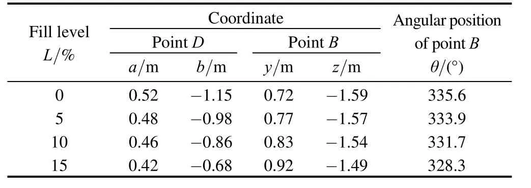
Table 4. Coordinates of point D and point B, the angular positions of point B for four levels of fill level

Fig. 8 shows a rule that the position of the maximum vibration point on the mill shell for higher fill level is at a lower angular position than that of lower fill level in the DEM simulation, which has a agree consistency with the result of the theoretical calculation.

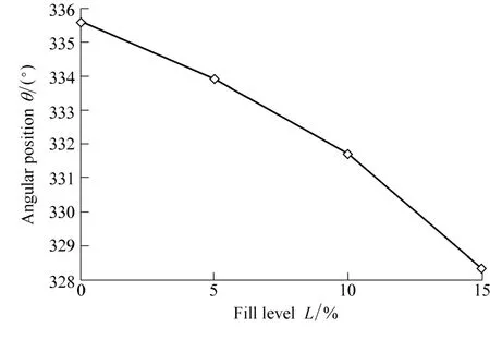
Fig. 8. Vibration in the angular position of the maximum vibration point on the mill shell with the fill level

4 Comparison between the Theoretical Calculation Results and DEM Simulation

Figs. 9–11 show the comparisons between the theoretical calculation and DEM simulated results. Due to the motion of the steel balls and coal in the DEM simulation, the accumulated height of the steel balls and coal at the bottom of roller is smaller than that of theoretical calculation at the same fill level. So the absolute values of z coordinate of the collision point (point D) in the DEM simulation is bigger than that of the theoretical results at the same fill level, and this conclusion can be observed from Fig. 9. Although at the same fill level the motion time of parabolic movement for ball C in the DEM simulation is shorter than that of theoretical calculation, the simulated velocity for detachment point in y direction is larger than that of theoretical value (see Table 2), and the absolute value of simulated y coordinate for detachment point is relatively smaller compared with that of theoretical value, which leads that the value of y coordinate for collision point is not smaller than that of theoretical value as shown in Fig. 9.

From the results presented in Fig. 9, it can be clearly seen that the absolute values of simulated y and z coordinates for collision point are all larger than those of theoretical values at the same fill level. However, the increased proportion of absolute value of the simulated y coordinate over the theoretical y coordinate for collision point is bigger than that of absolute value of z coordinate of collision point. So the y coordinate of the maximum vibration point that is calculated by the simulated y coordinate of collision point is lager than that of theoretical calculation, and the absolute value of z coordinate of this point is smaller than that of theoretical result, which can be seen in Fig. 10. And the angular position of the maximum vibration point in the DEM simulation is smaller than that of theoretical calculation at the same fill level as shown in Fig. 11.

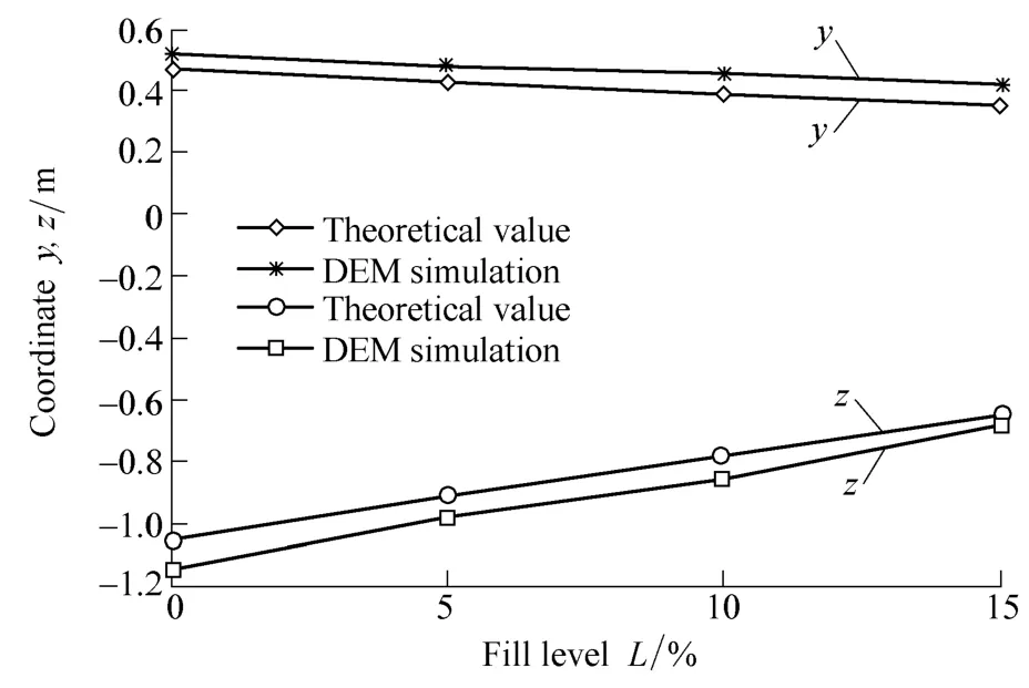
Fig. 9. Comparison between theoretical and DEM simulated coordinates (y and z) of collision point at various fill level cases

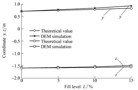
Fig. 10. Comparison between theoretical and DEM simulated coordinates (y and z) of the maximum vibration point on the mill shell at various fill level cases

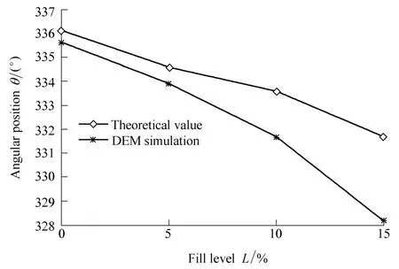
Fig. 11. Comparison between theoretical and DEM simulated angular position of the maximum vibration point on the mill shell at various fill level cases

5 Conclusions

(1)The angular positions of the maximum vibration point on the mill shell for different fill level cases are calculated theoretically under two assumptive conditions, respectively.The result shows that there is a descendent trend in the angular position of the maximum vibration point along with the increase of the fill level.

(2)The charge motion and power draft of the mill for different levels are simulated and predicted by the discrete element method. The simulated charge motion and power draft results are verified against the theoretical charge profiles and measured power drafts with an industrial ball mill, and then the DEM is validated to be very useful for simulating charge motion of the mill.

(3)Simulated motion trajectories of the steel ball in the outmost layer were tracked and analyzed to obtain the positions of the maximum vibration point on the mill shell.Having a same conclusion with result of theoretical calculation, the angular position of the maximum vibration point is lower for higher fill level than for lower fill level.

The angular position of the maximum vibration point may be utilized for measuring the fill level. However, this viewpoint needs to be validated further by processing the actual vibration signals that are collected from the mill shell. In the next work, a high resolution vibration sensor(accelerometer) will be mounted on the mill shell, and a lot of vibration signals will be collected under different experimental conditions and analyzed to verify the results of this paper.

[1] ZHANG Yiqiang. Coal level control for coal pulverizer using power(current) method[J]. East China Electric Power, 2001, 29(7): 48–49.(in Chinese)

[2] KOLACZ J. Measurement system of the mill charge in grinding ball mill circuits[J]. Mineral Engineering, 1997, 10 (12): 1 329–1 338.

[3] KANG E S, GUO Yugang, DU Yuyuan, et al. Acoustic vibration signal processing and analysis in ball mill[C]//Proceedings of the World Conference on Intelligent Control and Automation, Dalian,China, June 21–23, 2006: 6 690–6 693.

[4] SHA Yi, CAO Yingyu, GUO Yugang. Analysis of acoustic signal and BP neural network-based recognition of level of coal in ball mill[J]. Journal of Northeastern University, 2006, 27(12): 1 319–1 323. (in Chinese)

[5] XING Zhihao. Supervision and control of ball mill level indication realized by audio frequency signals[J]. Jiangsu Electrical Engineering, 2004, 23(4): 55–57. (in Chinese)

[6] BEHERA B, MISHRA B K, MAURTY C V R. Experimental analysis of charge dynamics in tumbling mills by vibration signature technique [J]. Minerals Engineering, 2007, 20(1): 84–91.

[7] LI Zunji, WANG Junrui, TANG Xinxi. An intelligent measuring and testing system of ball mill loading[J]. Electric Power, 2001,34(3): 45–47. (in Chinese)

[8] WANG Yingjie, LÜ Zhenzhong. Application study of bearing vibration signal in the load control system of tube mill[J]. Electrical Equipment, 2004, 5(9): 41–43. (in Chinese)

[9] CUNDALL P A, STRACK O D L. A discrete numerical model for granular assemblies[J]. Geotechnique, 1979, 29(1): 47–65.

[10] MISHRA B K, RAJAMANI R K. The discrete element method for the simulation of ball mills[J]. Applied Mathematical Modelling,1992, 16(11): 598–604.

[11] CLEARY P W. Predicting charge motion, power draw, segregation and wear in ball mills using discrete element methods[J]. Minerals Engineering, 1998, 11(11): 1 061–1 080.

[12] DONG H, MOYS M H. Assessment of discrete element method for one ball bouncing in a grinding mill[J]. Mineral Processing, 2002,65(3–4): 213–226.

[13] MAKOKHA A B, MOYS M H, BWALYA M M, et al. A new approach to optimizing the life and performance of worn liners in ball mills: experimental study and DEM simulation[J]. Mineral Processing, 2007, 84(1–4): 221–227.

[14] RAHMAN M K, MISHRA B K, RAJAMANI R K. Industrial tumbling mill power prediction using the discrete element method[J]. Minerals Engineering, 2001, 14(10): 1 321–1 328.

[15] MOYS M H, VAN N M A, VAN T J C, et al. Validation of discrete element method (DEM) by comparing predicted load behaviour of a grinding mill with measured data[C]//Proceedings of the XXI International Mineral Processing Congress, Rome, Italy,July23–27, 2000: 39–44.

[16] MISHRA B K, MURTY C V R. On the determination of contact parameters for realistic DEM simulations of ball mills[J]. Powder Technology, 2001, 115(3): 290–297.

[17] VENUGOPAL R, RAJAMANI R K. 3D simulation of charge motion in tumbling mills by the discrete element method[J]. Powder Technology, 2001, 115(2): 157–166.

[18] RAJAMANI R K, MISHRA B K, VENUGOPAL R, et al. Discrete element analysis of tumbling mills[J]. Powder Technology, 2000,109(1–3): 105–112.