Multidisciplinary Design Optimization with a New Effective Method

CHEN Xiaokai, LI Bangguo, and LIN Yi

National Engineering Laboratory of Electric Vehicle, Beijing Institute of Technology, Beijing 100081, China

1 Introduction

Collaborative optimization (CO) is a new design architecture to tackle the large-scale, distributed-analysis application often found in industry[1]. CO was originally proposed in 1994. It is one of several decomposition based methods that divide a design problem along disciplinary (or other convenient) boundaries. It consists of two-level optimization problems which are system optimization problem and subspace optimization problem. System optimizer optimizes the multidisciplinary variable (system level target)z to satisfy the interdisciplinary constraints while minimizing the system objective. Subspace optimizer minimizes the interdisciplinary compatibility constraints,while satisfying the subspace constraints. Relative to other decomposition-based methods, CO provides the disciplinary subspace with an unusually high level of autonomy[2].

The basic CO formulation is composed of system level and subspace level, the system level is given by Eq. (1)[2]:

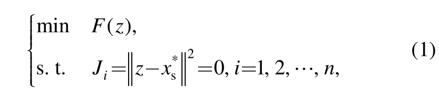
where F (z) is global objective, z is variable (i.e., system level targets for shared variables),is subspace target response that provides each subspace’s best attempt to meet the system level targets (z), and it is a parameter in system level, n is the number of subspaces.

The lower subspace level is illustrated in Eq. (2):

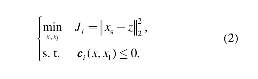
where x is an independent shared variable, xlis a local variable, which is relative only to the local subspace. On the basis of analyzing y = y (x, xl),y is coupling variable,is shared variable, z is a parameter,is a local constraint.

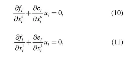
The subspace objective tries to match targets for the shared variables that have been sent by the system level[2].The dependent variables in subspace level include shared variables (xs) and local variables (xl). The shared variables include both independent variables (x) and coupling variables (y).

CO has been successfully applied to a variety of mathematical problems and engineering design problems，and used for the conceptual design of launch vehicles[3],high speed civil transports[4], and unmanned aerial vehicles[5]. However, the method also suffers from some challenges, which has been documented by ALEXANDROV, DEMIGUEL, et al[6–8]. They highlighted the features of CO that has an adverse effect on robustness and computational efficiency.

Three difficulties of the bi-level optimization problem stated in Eqs. (1) and (2) are considered.

(1) The system level Jacobian is singular at the solution[6]. This can be seen by noting that the constraint gradients are given byEven with a robust optimizer, this has an adverse impact on the rate of convergence.

(2) The Lagrange multipliers in the subspace problem are either zeroes or converge to zeroes as z converges toThis greatly affects subspace convergence.

(3) The subspace response ( Ji) is, in general, nonsmooth functions of the targets z[8]. As a result, the system level constraints are nonsmooth, hindering local and global convergence proofs for the system level problem.

In CO, the system compatibility constraints are equality constraints of quadratic forms, which often lead to some problems of convergence. Because of the quadratic equality constraints, CO also strongly depends on the initial condition for convergence. Inefficient convergence is often caused when gradient-based method is used.

The basic concept to enhance CO is to modify the system constraints, which cause the convergence difficulties[10]. The current research is focused on using the nature of the subspace problem, therefore the optimum constraints sensitivity is presented to find the closet point from the target point, while satisfying all disciplinary constraints.

2 Description of the Method

AZARM and LI[11]gave the formulation of a two level design optimization with an separable objective and separable constraints. The formation is given by Eq. (3) :

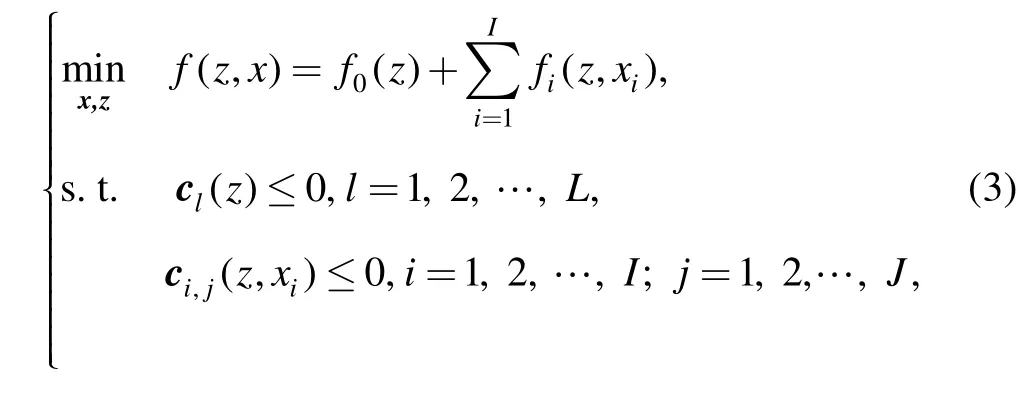
where f is an integrated objective function, fiis an objective function in subspace i.

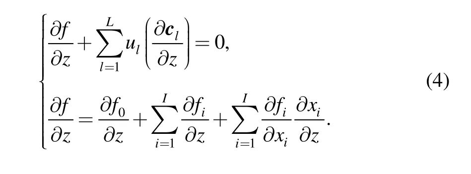
The Karush-Kuhn-Tucker (KKT) condition for this problem is given by Eq. (4):

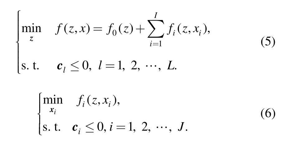
According to the two-level design optimization problem,CO can be written as another form. System level problem is given by Eq. (5), and subspace problems are given by Eq.(6):

The KKT optimality condition for subspace level optimization problem can be written as follows:

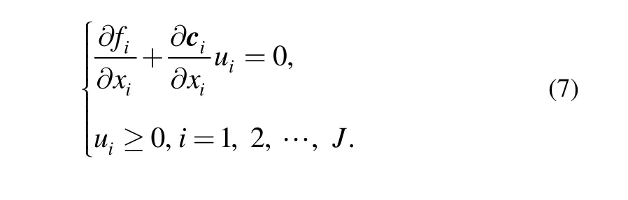
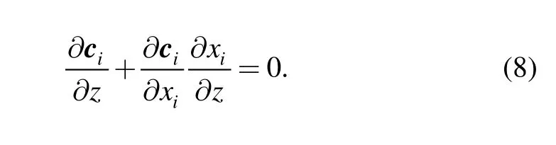
In CO, z is fixed and x is varied in subspace problem,we should have

Likewise, the KKT conditions for the system level optimization problem can be written as follows:

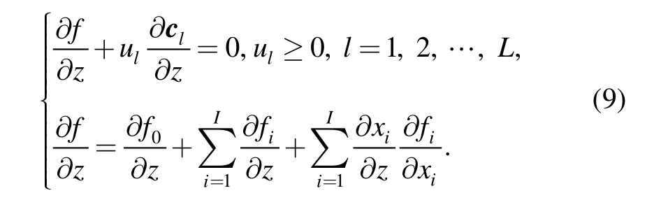
For CO, the variables in disciplinary optimization problem consist of shared variables and local variables, the KKT conditions for shared variables and local variables can be written as

CO synergizes the disciplinary problem via shared variables, according to Eqs. (4)–(9), a formulation can be obtained as follows:

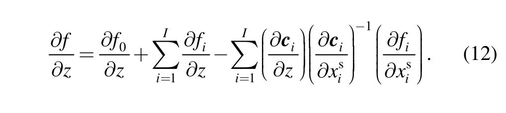
Once the shared variables have been identified, Eq. (12)can be used to obtain. Likewise, Eq. (12) can be used by an optimization method which does not yield the value of ui.

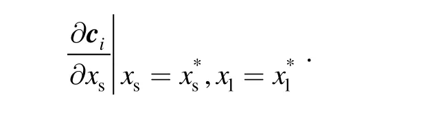
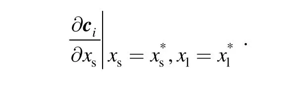
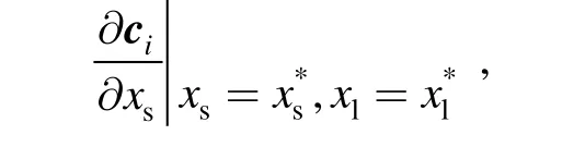
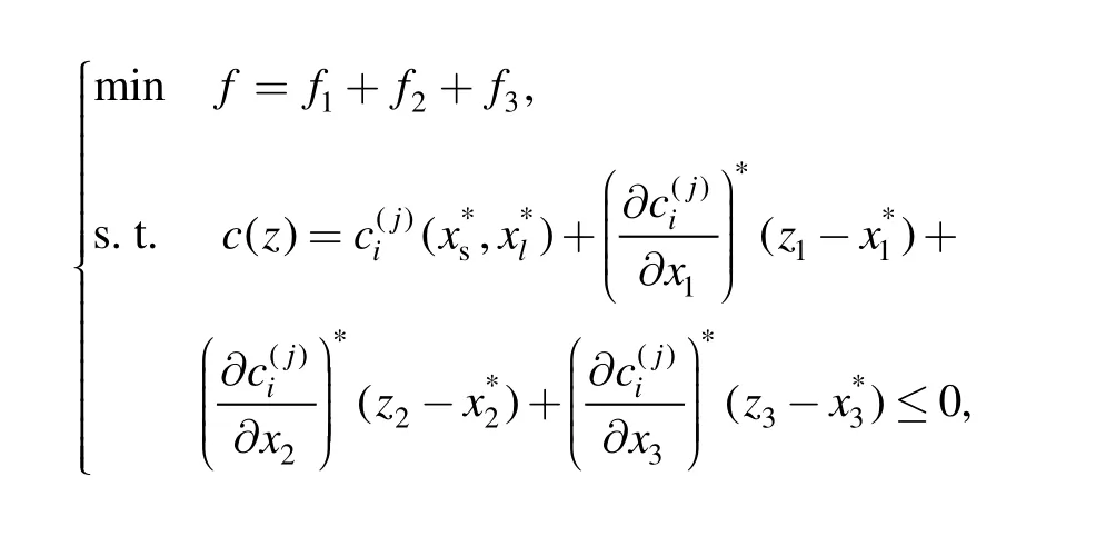
In CO, to modify the system level constraints, we define the derivative of local constraints while the variables areas the optimum sensitivity of disciplinary constraints according to the idea described above. That is

The optimum sensitivity of disciplinary constraints can reflect the changing information of disciplinary constraints,which enable the system level optimizer to know the boundary where the subspace objectives are zeroes.Through the optimum constraints sensitivity, the linear dynamic constraints of system level can be constructed by Taylor expansion around the subspace optimum as follows:

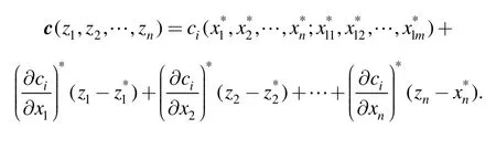
Where i is the number of disciplinary optimization problems, m is the dimension of local variables lx, n is the dimension of independent shared variables x.

These new constraints are linear constraints of variable z in system level, which can avoid the computational difficulties caused by the original quadratic equation constraints.is the constraint value when x = x*and, which is optimal value of each disciplinary optimization. Through these linear dynamic constraints, the optimized information of subspace optimization can be sent to the system level, which reinforces the exchange between system level and subspace level. The reformed CO is referred to as system level linear dynamic constraints collaborative optimization (DCCO).

3 Flow of DCCO

The solution process begins with an initial set of system level design variable z0. This variable is sent to the subspace optimization problems and treated as a set of fixed parameters. The subspace optimization problems are then solved while satisfying the subspace constraint ci.The parameterandare optimized in this optimization.

Then on the basis of

The system level optimizer determines whether the design variable z0satisfies the new constraints. Until now one whole optimization is finished. The process is repeated until z reaches the optimum.

4 Analytic Test Case and Application

This section illustrates the application of DCCO. The results of a typical functional optimization problem and a gear reducer optimization problem are compared with those obtained via the original version of CO. All problems were solved by sequential quadratic programming (SQP) method based on optimizer: NPSOL.

4.1 Typical function optimization problem

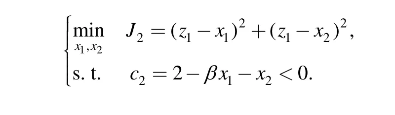
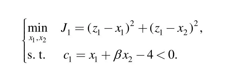
BRAUN[1]solved this typical function optimization problem via original version of CO. This problem is a constraint nonlinear problem, and its mathematical model is

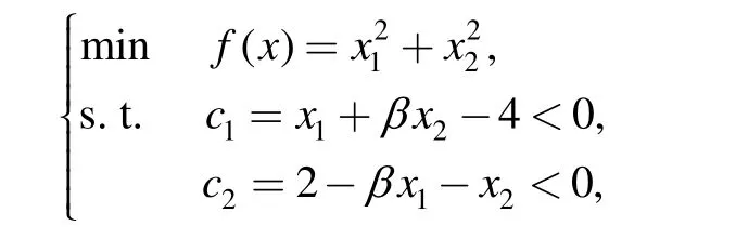
where β is a parameter, and β= 0.1. This problem is decomposed in the following manner. The system level problem and subspace level problem are described respectively.

The problem is solved by original version of CO, and system level problem is as follows:

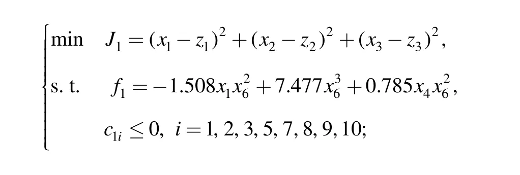
Disciplinary problem 1:

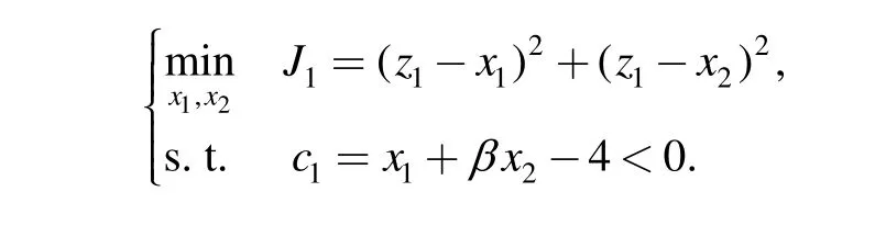
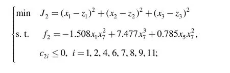
Disciplinary problem 2:

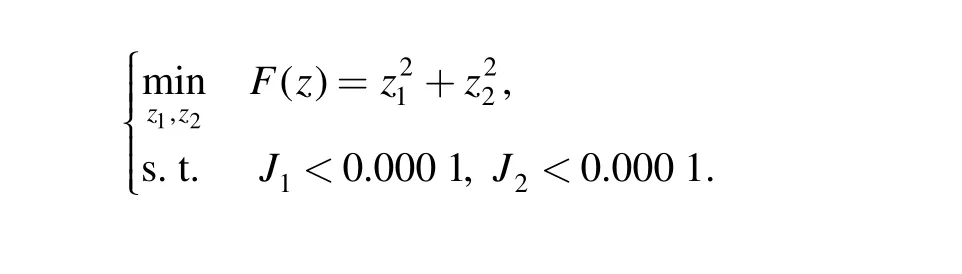
The problem is solved by DCCO, and the system level problem is as follows:

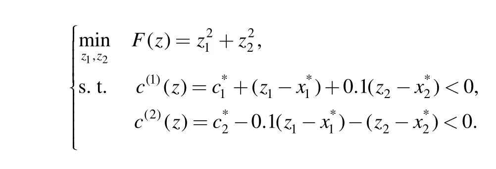
Disciplinary problem 3:

Disciplinary problem 4:

The results of this example are summarized in Table 1.For all cases, CO and DCCO methods could be used to solve this problem. Compared with CO of original version,the reformed method greatly reduces the number of the system level iteration. The results of this problem areand x2= 1.9 80. Conclusion can be drawn that the DCCO is more accurate than the original version of CO.

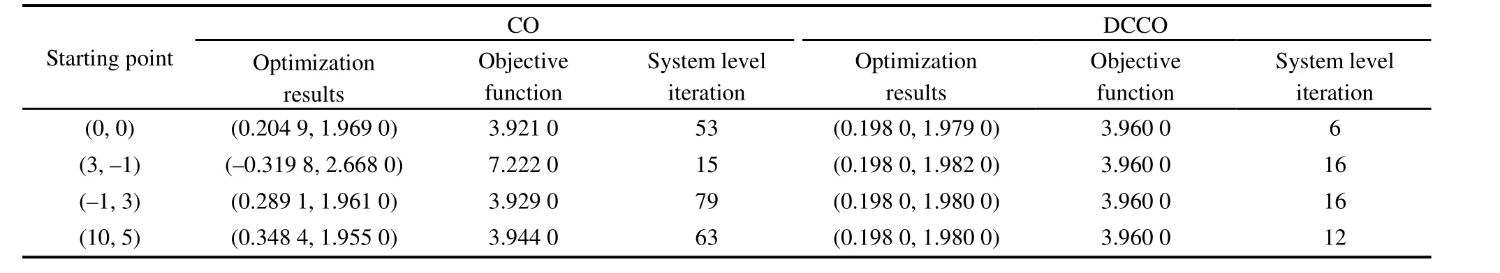
Table 1. Results of the typical function optimization problem solved by CO and DCCO

4.2 Example 2: gear reducer design problem

A well-known gear reducer example is presented in this section (see Fig. 1). The example is conducted to illustrate the effectiveness of this approach. The test problem is taken from AZARM, et al[11]. The objective of this optimization problem is to minimize the overall volume (or weight) of the speed reducer.

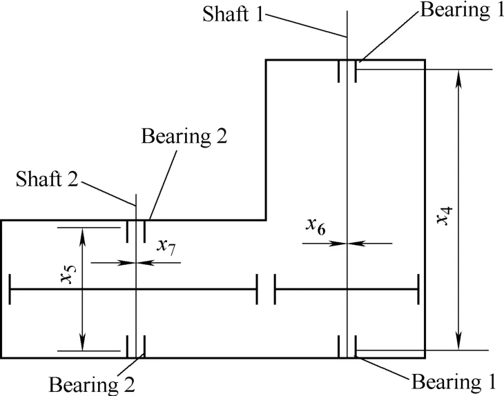
Fig. 1. Model of gear reducer example

There are 7 variables in this example, and the design variables are expressed as follows:

x1—Gear face width, 2.6 cm ≤ x1≤3.6 cm;

x2—Teeth module, 0.7 cm ≤ x2≤0.8 cm;

x3—Number of teeth of opinion, 17 ≤ x3≤28;

x4—Distance between bearing 1, 7.3 cm ≤ x4≤8.3 cm;

x5—Distance between bearing 2, 7.3 cm ≤ x5≤8.3 cm;

x6—Diameter of shaft 1, 2.9 cm ≤ x6≤3.9 cm;

x7—Diameter of shaft 2, 5 cm ≤ x7≤5.5 cm.

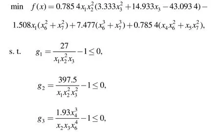
The nonlinear programming statement for this example is presented:

The gear reducer is decomposed into three disciplinary D1, D2, D3as follows:

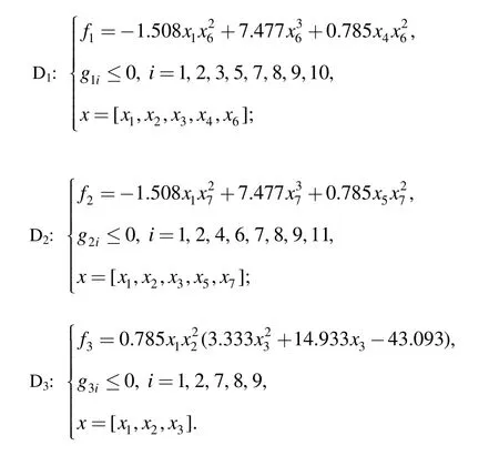
This problem is solved by DCCO, and the system level problem is as follows:

where i is the number of disciplinary problems,j is coupling constraints.

Disciplinary problem 5:

Disciplinary problem 6:

Disciplinary problem 7:

According to the range of design variables, choose X = (3.6, 0.8, 28, 7.3, 7.3, 2.9, 5.0) as the test design variable. The optimization process begins at X. Table 2 shows the summarized results of the given test design variables using DCCO method and CO method.

The original objective value is 6 533.6, after 25 iteration of system level optimizer, the objective function f (x)converges at 2 993.2, which is the final objective function value.

Table 2 also shows the summarized results of the given test design variables using CO method. The final objective function converges at 5 314.4, which is not the precise result of the optimization problem. AZARM, et al[12], gave the results of this problem. Design variables X is (3.5, 0.7,17, 7.3, 7.71, 3.35, 5.29), and objective function is 2 994.Now a conclusion can be drawn that the reformed collaborative optimization is effective to solve this multidisciplinary problem.

Fig. 2 gives the objective function iteration history via DCCO, which reveals the detailed convergence process.

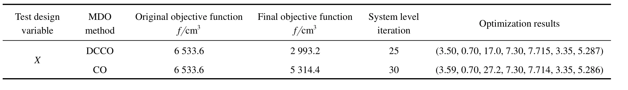
Table 2. Results of the gear reducer optimization problem via DCCO and CO

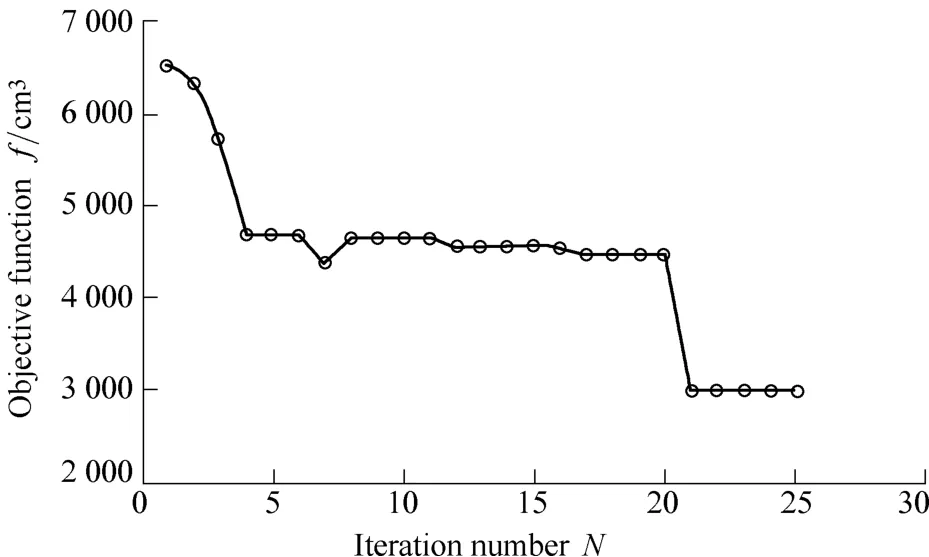
Fig. 2. Objective function iteration history via DCCO

5 Conclusions

(1) A new approach is investigated to modify collaborative optimization. The new approach is focused on making a breakthrough to find an approximate model of system constraints that allow system to converge faster and more robustly.

(2) A system-level linear dynamic collaborative optimization is presented by modifying the compatibility constraints of the original version of collaborative.

(3) Results of analytic analysis cases reveal that the reformed collaborative optimization can significantly improve system convergence and save computational time,compared to collaborative optimization. The price for this computational savings is a small increase in the complexity of constructing the system level constraints.

(4) The modified system level constraints are linear dynamic constraints, which can avoid some computational difficulties caused by the quadratic constraints contrast to the quadratic equality constraints of the original version of collaborative optimization.

[1] BRAUN R D. Collaborative optimization: an architecture for large-scale distributed design[D]. Palo Alto: Stanford University,1996.

[2] ROTH B, KROO I. Enhanced collaborative optimization: Application to analytic test problem and aircraft design[C]//12th AIAA/ISSMO Multidisciplinary Analysis and Optimization Conference,Victorian, British Columbia Canada, 10–12 September, 2008.

[3] BRAUN R, KROO I, MOORE A. Use of the collaborative optimization architecture for launch vehicle design[C]//6th AIAA/NASA/ISSMO Symposium on Multidisciplinary Analysis and Optimization, Reston, VA, Sept. 4–6, 1996.

[4] MANNING V. Larger-scale design of supersonic aircraft via collaborative optimization[D]. Palo Alto: Stanford University, 1999.

[5] SOBIESKI I. Multidisciplinary design using collaborative optimization[D]. Palo Alto: Stanford University, 1998.

[6] ALEXANDROV N M, LEWIS R. Analytical and computational aspects of collaborative optimization and multidisciplinary design[J]. AIAA Journal, 2002, 40(2): 301–309.

[7] ALEXANDROV N M, LEWIS R. Comparative properties of collaborative optimization and other approaches to MDO[M].Bradford: MCB University Press, 1999.

[8] DEMIGUEL A, MURRAY W. An analysis of collaborative optimization methods[C]//8th AIAA/USAF/NASA/ISSMO Symposium on Multidisciplinary Analysis and Optimization, Long Beach,CA, 2000.

[9] ALEXANDROV N M, LEWIS R. Engineering design optimization[M]. Bradford: MCB University Press, 1999.

[10] KOBAYASHI K, KROO I. The new effective MDO method based on collaborative optimization[C]//35th AIAA Fluid Dynamics Conference and Exhibit, 6–9 June, 2005, Toronto, Ontario Canada,AIAA Paper No. 2005–4799.

[11] AZARM S, LI W C. Optimality and constrained derivatives in Two-level Design Optimization[J]. ASME Journal of Mechanical Design, 1990, 112 (12): 563–568.

[12] AZARM S, LI W C. Multi-level design optimization using global momonicity analysis[J]. ASME Journal of Mechanisms and Automation in Design, 1989, 11(2): 259–263.