Development of a 2D spatial displacement estimation method for turbulence velocimetry of the gas puff imaging system on EAST

Letian LI (李乐天) ,Shaocheng LIU (刘少承) ,Ning YAN (颜宁) ,Xiaoju LIU (刘晓菊) and Xiang GAO (高翔)

1 Anhui University,Hefei 230039,People’s Republic of China

2 Institute of Plasma Physics,Chinese Academy of Sciences,Hefei 230031,People’s Republic of China

Abstract A gas puff imaging (GPI) diagnostic has been developed and operated on EAST since 2012,and the time-delay estimation (TDE) method is used to derive the propagation velocity of fluctuations from the two-dimensional GPI data.However,with the TDE method it is difficult to analyze the data with fast transient events,such as edge-localized mode (ELM).Consequently,a method called the spatial displacement estimation (SDE) algorithm is developed to estimate the turbulence velocity with high temporal resolution.Based on the SDE algorithm,we make some improvements,including an adaptive median filter and super-resolution technology.After the development of the algorithm,a straight-line movement and a curved-line movement are used to test the accuracy of the algorithm,and the calculated speed agrees well with preset speed.This SDE algorithm is applied to the EAST GPI data analysis,and the derived propagation velocity of turbulence is consistent with that from the TDE method,but with much higher temporal resolution.

Keywords: gas puff imaging,spatial displacement estimation,SDE,edge turbulence velocity,TDE,EAST tokamak

1.Introduction

The edge turbulence can contribute to remarkable cross-field transport in magnetically confined plasmas,such as blobs or filaments [1-3].During the propagation of blobs from the plasma edge to the scrape-off layer (SOL),a large amount of heat and numerous particles across the last closed flux surface (LCFS) can reach the divertor plates in a short time and lead to heat deposition on the first plasma-facing materials.Some fast transient events,such as edge-localized mode(ELM) can cause significant energy loss in the core plasma and high heat flux at the divertor target,which is a crucial issue for large fusion devices such as ITER.Consequently,the fine dynamic evolution of the edge turbulence is important for understanding edge cross-field transport and core plasma confinement.

Two-dimensional (2D) imaging technology is applied to the measurement of edge turbulence structure and its propagation velocity.Several 2D diagnostics for turbulence structure have been developed,including beam emission spectroscopy (BES) [4-6 ],Langmuir probe [7-9],electron cyclotron emission imaging (ECEI) [10-14] and gas puff imaging (GPI) [15-17].The Langmuir probe array inserted into the edge plasma can measure floating potentials and ion saturation current directly,providing the turbulence information with high temporal evolution [18].The BES and ECEI can measure the edge 2D turbulence structure via the light emission and microwave,respectively.The GPI measures the 2D edge turbulence by injecting neutral gas (helium or deuterium) and capturing the line emission with a high-speed camera.Many tokamaks are equipped with GPI diagnostics,such as NSTX [19],Alcator C-Mod [20],TEXTOR [21],HL-2A [17] and J-TEXT [22].

Since the turbulence flow velocity is an essential parameter for the understanding of turbulence instability and radial transport,various methods are used in velocity estimation,such as the time-delay method (TDE) [23],optical flow [24],orthogonal dynamics programming (ODP) [25] and spatial displacement estimation (SDE) [26].For example,velocity analysis for the BES diagnostic on DIII-D is performed using the ODP method [27].Velocity calculations for the Langmuir probe on NSTX and ECEI diagnostic on KSTAR are done using TDE estimation [28,29].In the TDE process,cross-correlation is performed between a reference point and the surrounding points in a series of time sequences,and the displacement is given by the distance between the two points with the maximum cross-correlation coefficient.Finally,the speed is estimated by the ratio of displacement and delay time.The velocity calculated by the TDE method has high precision,and its spatial resolution can reach optical resolution.However,time series data are required for TDE analysis,and it is difficult for this analysis to provide precise velocity in a situation with large-scale motion during a short time period.The optical flow method estimates the speed by detecting the light change on a target object.This method requires constant brightness on the target object,which is a challenge for the GPI image.In addition,if the movement is too fast and the specific structure exceeds the observation window,the optical flow method will fail to attain the correct speed,which is called the aperture problem.The SDE method calculates the spatial displacement from the spatial lag of the 2D spatial cross-correlation coefficient function.Since the SDE can be operated for two adjacent images,it has much higher temporal resolution than the TDE method,which is an advantage for the velocity estimation of fast structures.Due to the SDE method needing enough large image pixels,its spatial resolution is limited.

Some improvements are added to the SDE algorithm that is applied to the GPI data analysis on EAST.First,we introduce an adaptive median filter [30],which can effectively solve the filtering problem when the noise is relatively high.The window size of the median filter can be dynamically modified according to the preset conditions,aiming to denoise and simultaneously preserve the detailed information of the signal.Second,the super-resolution reconstruction by bicubic upsampling [31] is used to acquire high spatial resolution image data and easily extract the detailed structure.Third,the location of a specific structure is captured automatically using an appropriate window size according to the structure's peak.When we finish the development of the SDE algorithm,it is tested by two given motion trajectories,exhibiting accurate moving speed.Finally,the SDE method is applied to the GPI data analysis,and the calculated velocity agrees well with that from the TDE method.The imaged frame can be split into 20×30 pixel2sub-frames.Therefore,the velocity distribution in the poloidal-radial plane is obtained.The rest of this paper is organized as follows.Section 2 is the development of the SDE algorithm,and the corresponding test and application on GPI data are presented in section 3 .Section 4 is a summary.

2.Development of SDE algorithm

In this section,we introduce the SDE algorithm in detail.The algorithm includes the following steps: data pre-processing,image enhancement,speed estimation.The purpose of data pre-processing is to remove background noise and the motion trend.Image enhancement can improve the quality and visibility of images that are easy to analyze and understand.Adaptive median filtering can help us to reasonably process the signal noise under different noise levels,preserve image details and make the subsequent calculations more accurate.Super-resolution processing can increase the image’s resolution,thereby improving the details and clarity of the picture.Using super-resolution processing technology,we can convert a low-resolution image into a high-resolution image,consequently enhance the quality of the image.The third step is to convert the time-domain signal into a frequency-domain signal through fast Fourier transform(FFT) [32],perform cross-correlation operations,and obtain the displacement from the polynomial fitting.Finally,the velocity is calculated by the relative displacement and the delay time.

2.1.Pre-processing

In this part,we preprocess the GPI data.First,since the background radiation will disturb the turbulence motion in GPI images,the background emission should be removed in the pre-processing stage.The background emission is given by the average of a series of frames before the helium gas reaches the edge plasma,and then every frame subtracts the background emission to remove the background [15].The original GPI image is shown in figure 1(a),and the background light radiation intensity before gas puffing is presented in figure 1(b).When we remove the background emission intensity from the original 2D signal,we obtain figure 1(c).Finally the fluctuations of the GPI emission intensity are derived by subtracting the averaged emission intensity of the interested GPI frames (t=3.466925-3.467121s) from figure 1(c),as shown in figure 1(d).

Detrending refers to removing some information in the image sequence that affects the speed estimation [33],such as signal offset.Detrending is an essential part of speed estimation because it can further improve the velocity estimation accuracy.After the background removal step,we detrend the data usingnth-order polynomial fitting,as presented in reference [26].The images before and after the polynomial detrending are shown in figures 2(a) and (b) for discharge #102993,respectively.The trend is much lower than the signal level,as illustrated in figure 2(c).

Figure 1.(a) Original GPI image measured in discharge #102993,(b) background emission intensity before gas puffing,(c) the same image after removing the background emission,(d) the image with the averaged emission intensity subtracted.

Figure 2.(a) The image before detrending,(b) the image after detrending,(c) the trend of image calculated by the nth-order polynomial fitting.

2.2.Image enhancement

2.2.1.Adaptive median filteringThe median filter is widely used in image processing [34].The median filter works by calculating the median value of the pixels in the neighborhood of each pixel and assigning this value to the central pixel.Compared to other filtering methods,the median filter is an effective way to remove noise from images and simultaneously preserve edge information without remarkable blurring.This makes it a widely-used tool in the field of image processing.

If a larger filter window is used for the median filter,it can effectively remove noise,but it also leads to a fuzzy image that is unfavorable in the subsequent calculations.Conversely,using a smaller filter window can help preserve more details and enhance the clarity of the image,but it is not an effective way to remove noise.Therefore,an adaptive median filter is adopted to dynamically modify the window size based on the noise level [30].

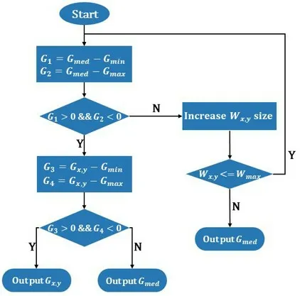
Figure 3.Workflow diagram of the adaptive median filter.

The adaptive median filter can dynamically change the window size of the filter according to the preset conditions.The filtering is performed on a point (x,y) of the image and inside a rectangular windowWx,y,with an allowed maximum window size ofWmax.Gx,yrepresents the gray value of point (x,y) .Gmed,GminandGmaxare the median,minimum gray value and maximum gray value in the window (excluding point (x,y)),respectively.The working principle of the adaptive median filter is illustrated in figure 3.In the first diamond,we use the intensity ofG1andG2to determine whether the gray median value in the window is too large or too small.IfGmedis betweenGminandGmax,the window size is appropriate.Next,we determine whether the valueGx,yis noise;ifGx,yis beyond the range fromGmintoGmax,the window size should be expanded.As shown in the second diamond,if the gray valueGx,yis also within a reasonable range,we consider that this point is not noise,and outputGx,y;if the point is not within a reasonable range,we consider it to be noise,and outputGmed.If the window size needs to be enlarged after the first diamond,we will increase the window sizeWx,y,then determine whether the new window size exceeds the maximum valueWmax.If not,we return to “Start”,otherwise we outputGmed.

2.2.2.Super-resolutionThe upgrade of the GPI system on EAST was completed in 2021 [35].In the upgraded optical system,the high-speed camera has a speed of up to 531645 frames/s and the captured image has a resolution of 128×64 pixel2.When estimating the velocity of the turbulence structure,we extract the image matrix of the structure and its surroundings (approximately twice the structure length in total) and minimize the influence of movement from the outside area.To achieve both high accuracy and smoothness of the image detail,bicubic upsampling super-resolution processing is adopted to extract image data [31].In the bicubic interpolation algorithm,we assume that the interpolation at a certain pointp(x,y) is obtained by weighting the four points around it,which can be written as follows:

The interpolation kernel function is:

The interpolation result ofp(x,y) is:

Assume that pointp(x,y) is located in the original image at the position shown in figure A1,where Q is the matrix of pixel values of the 16 nearest points top. Wxand Wyare calculated by the interpolation kernel function in thexdirection andydirection ofp:

Rpis the interpolation value of pointpand calculated by multiplying the three matrices of Wx,Q and.In equation (2),ais set as a constant and the default value is -0.5 [31].The specific derivation process is shown in the Appendix.

For example,we extract the turbulence structure of one GPI frame for super-resolution testing,as shown in figure 4.The reconstructed image with bicubic upsampling exhibits smoother shape edge and a clearer structure compared to the original image.

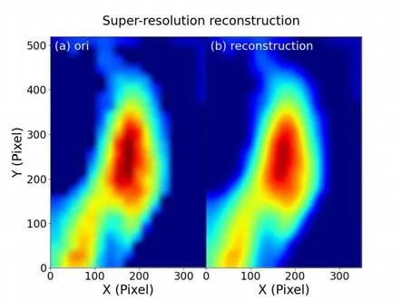
Figure 4.(a) The original image,(b) the reconstructed image enlarged ten times with bicubic upsampling.

2.3.Speed estimation

2.3.1.Fast Fourier transformFourier transform has been used in various fields of engineering and science.Fourier transform converts images from the spatial domain to the frequency domain,enabling efficient and accurate image analysis.Fast Fourier transform (FFT) [32] is an efficient algorithm of discrete Fourier transform (DFT) [36] and is more suitable for handling large-scale signals or images than DFT.Compared to DFT,FFT incorporates a recursive algorithm based on the divide-and-conquer strategy,which enhances the speed of Fourier transform calculations.The FFT algorithm reduces the computational complexity of DFT fromO(n2) toO(nlogn),and this reduction in complexity allows for faster computation of Fourier transforms.In image processing,FFT plays a significant role in transforming an image from the spatial to the frequency domain.For the discrete 2D Fourier transform of an image with sizeM×N,the equation is as follows:

whereF(u,v) is the value in the frequency domain,Mis the width of the image,Nis the height of the image,f(x,y) is the value in the spatial domain,iis the imaginary unit,xandyare pixel coordinates,uandvrepresent the horizontal and vertical coordinates in the frequency domain,the value range ofuis 0 ≤u≤M-1,and the value range ofvis 0 ≤v≤N-1.

2.3.2.2D cross-correlationCross-correlation has many applications in signal and image processing.2D cross-correlation,which computes the correlation coefficient between two images in the spatial domain,is commonly used in searching for similar structures among images,image alignment and image registration.In the SDE method,2D crosscorrelation is used to estimate the relative shift [26],as defined by:

whereA,B*are 2D signals in frequency-domain obtained using the FFT process,B*is the complex conjugate ofBandF-1denotes the inverse Fourier transform operation.φ(x,y)is the circular 2D cross-correlation function.Since convolution in the time or spatial domain can be expressed by frequency domain multiplication,and correlation is a form of convolution,we express correlation by frequency-domain multiplication [37].The location of the largest correlation can be found at the maximums of φ(x,y) [38].

Taking two consecutive frames as an example,first,the cross-correlation operation is carried out between the original frame and itself,in order to obtain the relative initial position of the target structure,namedPori.Next,the crosscorrelation between the two frames is calculated to find the point with the maximum coherence value,namedPc.Finally,the relative displacement is given by the Euclidean distance betweenPoriandPc[39].

The EAST GPI images of discharge #102993 after the pre-processing and adaptive median filtering are shown in figure 5.A bright eddy structure is in the middle of the images,and clear propagation is observed in the time sequence of the images.In order to illustrate the 2D crosscorrelation method,two images from figures 5(i) and (p) are selected to perform the FFT and 2D cross-correlation analysis.The 2D cross-correlation spectrum is converted back to the spatial domain by inverse FFT,and the results are shown in figure 6.Comparing the self-correlation of the first frame with the cross-correlation between frames (i) and (p) in figure 5,the coordinates of the pointsPoriandPccan be fixed,and a clear relative displacement between them is observed,which is consistent with the direction of movement in figure 5.

2.3.3.Sub-pixel precision processingThe accuracy of the relative displacement derived fromPoriandPcin the previous section is at pixel level.The image recorded by the GPI high-speed camera is 64×128 pixel2on EAST,and the pixel area occupied by the turbulence structure is small.In order to improve the calculation accuracy,a second-order polynomial fitting is used to fit the location with the maximum correlation coefficient and its surrounding area.Consequently,the maximum correlation position can be obtained with sub-pixel accuracy [26].The fitting equation is:

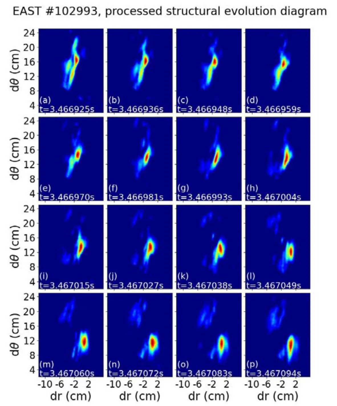
Figure 5.Time sequences of GPI image after the pre-processing and adaptive median filtering.The corresponding time slices are annotated in panels (a) to (p).

Figure 6.(a) The cross-correlation operation between the first frame (panel (i) of figure 5) and itself,(b) the cross-correlation calculation between the second frame (panel (p) of figure 5) and the first frame.

whereai(i=0,1,2,3,4,5) is the fitting coefficient andx,yare coordinates in the cross-correlation spectrum.The position with the maximum correlation coefficient is calculated by the partial differentiation ofxandywith polynomial fitting in equation (9),and the calculated position is given by:

2.3.4.Velocity calculationFrom the obtainedxmaxandymax,a more accurate relative displacement betweenPoriandPccan be calculated.The coordinates of pointsPoriandPcare(xmax1,ymax1) and (xmax2,ymax2) respectively,and the Euclidean distance between these two points can be expressed as:

Finally,the speed of movement can be estimated from the relative displacementdand the delay time τ.

3.Application of SDE algorithm

3.1.Algorithm test

In this section,the validity and accuracy of the SDE algorithm are tested.Two types of motion trajectories are used in the test,with a linear motion and a curvilinear motion,as illustrated in figure 7.The frames are set at 137×159 pixel2,which is similar to the GPI rotated image of EAST.The time period of these two movements is set at 5 s,with an interval of 0.1 s between two adjacent frames.For the linear motion,the elliptical structure moves along the diagonal straight line,with a constant shape and direction.For the curvilinear motion,the trajectory is a curve,and the shape and tilted angle of the red structure change gradually frame by frame.The moving velocity calculated by the SDE algorithm is presented in figure 8.For both movements,the calculated velocities agree well with the preset velocities.The velocity of the linear motion has symmetrical distribution,i.e.the red structure accelerates first and then decelerates with the same accelerated speed.The results of both cases demonstrate that the SDE algorithm is valid and its accuracy is very high.

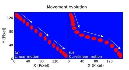
Figure 7.Motion trajectories.(a) A linear motion,(b) a curvilinear motion.The speed in both cases is first accelerated and then decelerated.

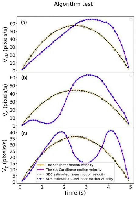
Figure 8.The structure velocity for the straight and curvilinear motions was calculated by the SDE method.(a) Two-dimensional velocity,(b) velocity in the x-direction,(c) velocity in the y-direction.

3.2.GPI data analysis

The SDE algorithm is applied to the GPI data analysis in EAST for discharge #103882.The GPI diagnostic is operated with a frame rate of 531645 Hz and an interval of 1.88μs between two adjacent frames.As a reference,the turbulence propagation velocities in the radial and poloidal directions are calculated using the TDE method,with a velocity point derived from 50 continuous frames,as shown in figure 9.Around the LCFS,the turbulence radial velocityVris mainly directed outwards with a maximum value of about 2 km/s.The turbulence poloidal velocityVθis directed in the ion-diamagnetic drift direction in the SOL and in the electro-diamagnetic drift direction inside the LCFS,with a maximum value of over 3 km/s.During the L-H transition on NSTX,turbulence poloidal velocity was also observed to propagate towards the electron diamagnetic drift direction inside the LCFS [40,41].Note that the event at 8.6256 s is the eruption of an ELM burst.The turbulence velocities are also calculated using the SDE algorithm in the same time period as the TDE method,as illustrated in figure 10.The GPI image is divided into 6×6 sub-frames,with 20×30 pixel2for each sub-frame.In contrast with the TDE method,the radial velocityVrin figure 10(a) exhibits clear outward propagation around the LCFS,which is similar to that in figure 9(a).Note that theVrfrom the SDE method reveals more details of the variation due to its high temporal resolution.The poloidal velocityVθin figure 10(b) reveals the same radial distribution as the TDE method in figure 9(b).Due to the high temporal resolution of the SDE algorithm,the dynamic evolution ofVθis observed within the 550μs period,and the significant changes inVθare consistent with the peaks of the divertor Dαsignal,indicating the correlation between upstream turbulence and downstream particle deposition.During the ELM burst,a significant increase is detected in the Dαsignal,with numerous particles moving outwards across the magnetic field lines.At the same time,high turbulence propagation velocity is observed onVrandVθin figures 9 and 10.In summary,the SDE algorithm reveals similar velocity estimation results to the TDE method,but has much higher temporal resolution.

4.Summary

The SDE algorithm is developed and applied to the GPI diagnostic on EAST tokamak.The SDE algorithm includes pre-processing,adaptive median filtering,super-resolution,2D cross-correlation via FFT,and displacement estimation.In these procedures,we remove the background and noise from the image data and preserve the detailed information of the structure.The computation efficiency is high because FFT is introduced into the 2D spatial cross-correlation technology.The temporal resolution of the SDE algorithm is as high as the temporal resolution of the GPI diagnostic,which is a significant advantage for the velocity analysis of fast events.The developed SDE algorithm is tested with a linear motion and a curvilinear motion,and the derived velocities agree with the preset velocities with high accuracy.The new SDE algorithm is applied to the GPI data analysis on EAST,and the calculated propagation velocity of turbulence is consistent with that from the TDE method,but has much higher temporal resolution.Due to its precision and high temporal resolution,the SDE method can estimate the propagation velocity of turbulence in fast transient cases,such as the eruption of ELM and other instabilities.Consequently,the SDE method provides an effective way to analyze the 2D image data with fast variations,which is important for the understanding of edge turbulence in fusion devices.

Figure 9.The turbulence propagation velocities calculated using the TDE method for discharge #103882.(a) Radial velocity,with positive value directed outside,(b) poloidal velocity,with positive value directed upwards (electron-diamagnetic drift direction).The purple dashed line represents LCFS.

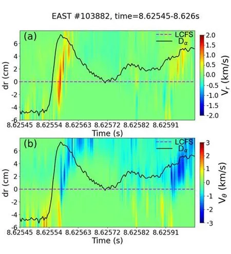
Figure 10.Turbulence propagation velocities calculated using the SDE algorithm.(a) Radial velocity,(b) poloidal velocity.The temporal variations of a Dα signal are shown in panel (b).The time traces of GPI signal and Dα signal are aligned by some fast events.The purple dashed line represents LCFS.

Acknowledgments

This work was supported by the National Magnetic Confinement Fusion Energy R&D Program of China (Nos.2022YFE03030001,2022YFE03020004 and 2022YFE 03050003),National Natural Science Foundation of China(Nos.12275310,11975275,12175277 and 11975271),the Science Foundation of Institute of Plasma Physics,Chinese Academy of Sciences (No.DSJJ-2021-01),the Collaborative Innovation Program of Hefei Science Center,Chinese Academy of Sciences (No.2021HSC-CIP019) and the Users with Excellence Program of Hefei Science Center,Chinese Academy of Sciences (Nos.2021HSC-UE014 and 2021HSCUE012).

Appendix.Bicubic upsampling

We developed a coordinate system to demonstrate the calculation process by the kernel function in equation (2).

Figure A1.Interpolation process in super-resolution processing.

The coordinates of pointpare (xp,yp),and the interpolation result isRpand the distance from the point to nearby pixels is Δxand Δy.If 0<Δx<1,then 1<Δx+1<2,-1<Δx-1<0,-2<Δx-2<-1.Therefore,from equation (2) we obtain:

Equation (5) can be derived from the equations listed above.