An improved TDE technique for derivation of 2D turbulence structures based on GPI data in toroidal plasma

Weice WANG (王威策) ,Jun CHENG (程钧) ,Zhongbing SHI (石中兵) ,Longwen YAN (严龙文) ,Zhihui HUANG (黄治辉) ,Kaiyang YI (弋开阳) ,Na WU (吴娜),Yu HE (何钰),Qian ZOU (邹千),Xi CHEN (陈熙),Wen ZHANG (张文),Jian CHEN (陈建),Lin NIE (聂林),Xiaoquan JI (季小全) and Wulyu ZHONG (钟武律)

1 Southwestern Institute of Physics,Chengdu 610299,People’s Republic of China

2 Institute of Fusion Science,School of Physical Science and Technology,Southwest Jiaotong University,Chengdu 610031,People’s Republic of China

Abstract This paper reports an improved time-delay estimation (TDE) technique for the derivation of turbulence structures based on gas-puff imaging data.The improved TDE technique,integrating an inverse timing search and hierarchical strategy,offers superior accuracy in calculating turbulent velocity field maps and analyzing blob dynamics,which has the power to obtain the radial profiles of equilibrium poloidal velocity,blob size and its radial velocity,even the fluctuation analysis,such as geodesic acoustic modes and quasi-coherent mode,etc.This improved technique could provide important 2D information for the study of edge turbulence and blob dynamics,advancing the understanding of edge turbulence physics in fusion plasmas.

Keywords: gas-puff imaging,TDE method,turbulence,velocity field map

1.Introduction

The scrape-off layer (SOL) in a tokamak is known to exist blobs or filaments [1],which are elongated structures along the magnetic field lines with a much higher density than the background plasma [2].These structures are intermittent and contribute significantly to radial transport outside the last closed flux surface (LCFS) [3,4].These structures and smallscale turbulence together determine anomalous thermal and particle transport at the boundary and affect the SOL width.Therefore,studying these structures is crucial for understanding plasma-wall interactions (PWI) [5,6].Turbulent structure measurements of tokamak plasmas,especially in the boundary region,have been performed for decades,but they are mainly limited to single-point or one-dimensional(1D) measurements,such as Langmuir probes.Langmuir probes have traditionally been used to identify filament structures by measuring plasma fluctuations.However,the high heat load can damage probes and release impurities that pollute the plasma.In contrast,a gas-puff imaging (GPI)system,which is a diagnostic system for measuring the instantaneous two-dimensional (2D) structures of the turbulence at the boundary of magnetically confined plasmas,provides non-invasive observation with a wide and flexible view region and good spatial resolution by measuring visible light emission from boundary plasma [7,8].The 2D images obtained by the GPI system are processed using the time-delay estimation (TDE) technique to obtain velocity fluctuation map of turbulence or shear flow.The basic TDE technique,based on cross-correlation and wavelet analyses with gradient algorithm,has been applied in many tokamaks to analyze diagnostic data.

In past studies,the TDE technique was applied to analyze 1D signals from beam emission spectroscopy (BES)diagnostic to measure the turbulence flow field in DIII-D tokamak [9-12].It has also been used to derive time-dependent 2D velocity field maps based on normal optical flow on NSTX [13].Another TDE technique based on dynamic programming has been proposed to process BES data and analyze velocimetry during L-H transition from GPI 2D signals in EAST tokamak [14].Recently,a 2D time-delay cross-correlation technique has been used to analyze zonal flow on Alcator C-Mod [15].However,these techniques do not completely address the limitations caused by the aperture problem,variable inter-frame shifts,sudden changes in brightness,one-way timing delay,and reconstruction of lowfrequency signals.To overcome these limitations,an improved TDE technique based on dense optical flow technique is applied to analyze 2D GPI signals such as velocity field map and MHD-correlated blob [16,17].It has advantages in improved accuracy,robustness to large displacements,handling of occlusions.The improved technology adaptively identifies blobs and tracks their movement,recording the number of blobs,velocities,and other dynamic characteristics.The derivation of the velocity field maps by the TDE technique is important for the understanding of turbulence,blobs-related radial transport and the determination of the poloidal flow pattern at the boundary plasma.

In this study,poloidal and radial fluctuation velocitiesVθ,Vrare obtained directly by the TDE technique,poloidal shear flow is defined as ∂Vθ/∂r,Reynolds stress is also calculated by .The organization of this paper is as follows.Section 2 introduces the blob tracking method and velocity field technique,including imaging modeling and main steps of the improved TDE technique.Preliminary experiment results are shown in section 3.Section 4 is the summary.

2.Improvement of TDE technique

2.1.Image modeling

The raw 2D digital signals taken by the camera need some processing to restore the physical information.The following methods are only for 2D greyscale images.We propose a simple yet effective background removal algorithm for lowresolution grayscale GPI data based on running average background subtraction.The algorithm assumes a relatively static background and minimal camera movement,making it well-suited for control environments.By continuously updating a running average background model with a user-defined learning rate modified in different plasma discharges,the algorithm adapts to gradual changes in the scene.The learning rate can be tailored based on specific parameters of plasma discharges.For instance,in high confinement mode discharges,a lower learning rate may be employed to avoid noise whereas in ohmic or low confinement mode discharges,higher rates might be preferable to capture rapid coherent structural changes.While the proposed model is adaptable to a variety of plasma discharge conditions simply by tweaking the learning rate,certain extreme or unique scenarios might benefit from alternative models or additional preprocessing.Nonetheless,for the bulk of scenarios we examined,adjusting the learning rate should be reasonable.The foreground is extracted by computing the absolute difference between the current frame and the running average background,followed by thresholding to generate a binary foreground mask.This method offers a computationally efficient solution for background subtraction in lowresolution grayscale GPI images,while maintaining the ability to adapt slow background variations.It is helpful to solve the interference of vacuum chamber components on imaging.

Next,each frame in the original data is filtered with convolution kernel to remove the noise of an image.Compared with median and Gaussian filters,the convolution kernel filter,such as a high pass filter kernel and Bilateral Blur [18,19],can reduce spurious spikes of the images,it can better retain the original structure relationship of the images,primary intensity and sharpen images,which is beneficial to observe the large-scale structure of boundary plasma.In addition,the convolution kernel can be adjusted freely for different image features.In this work,due to the significant difference between the discharges,different convolution kernels are used for processing different discharge conditions.The convolution kernel is not adaptive and determined by the electron temperature and density of the boundary plasma.This process can be particularly effective for regions with a low signal-to-noise ratio (SNR),as the calculation of velocity is highly sensitive to spurious spikes in the 2D data.

To ensure the assumption of constant brightness and identical time intervals between frames,some frames are merged when the brightness of more than two consecutive frames is below half of the average brightness of this discharge,meanwhile,the local brightness must be normalized to the average brightness.This step is accomplished by simply normalized brightness for each frame using the average brightness of all frames.After the above steps,a set of pixel matrices of the same time intervals is obtained.The velocity field is calculated based on this set of matrices.Besides,the signal of pixel in the same position of successive frames can partially approximate to the fluctuation signal of the saturation ion current measured by Langmuir probes in the SOL.

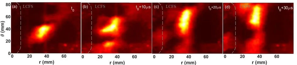
Figure 1.A set of GPI images taken with an exposure time of 10 μs during a typical discharge.The poloidal (vertical) scale “θ” is only indicated in the first frame,and the radial scales “r” are indicated in each frame.The electron diamagnetic direction is towards the top.The radial outward direction is towards the right side.

2.2.Blob tracking

This section presents a comprehensive approach for detecting,tracking,and characterizing blob-like structures within GPI data.The proposed technique consists of seven interconnected steps.(i) The image is scanned row-wise from the topleft corner to identify blob trigger frames,using a predefined blob tracking trigger threshold and the number of pixels (N) above this threshold for statistics.(ii) When the number of pixels over the threshold exceeds the specified assumption value,a blob is triggered within the frame,and the value is constrained by the radial position of the SOL.(iii) A connected region recognition algorithm is then employed to determine the maximum brightness pixel in the triggered frame,which serves as basic pixel point.Adjacent pixels are iteratively examined to verify if they meet the threshold condition,and the deriving connected region represents the outline of one or multiple blobs.(iv) To ensure the continuity and separability of blob contours across frames,the Hausdorff distance [20] method is utilized to compare contour similarities.(v) Similar outlines are grouped into a blob sequence,while dissimilar outlines are separated.This similarity comparison allows the algorithm to track multiple blobs within a single frame.(vi) Only blobs persisting for at least three frames are retained for further analysis,effectively eliminating noise and transient features. After completing the aforementioned steps,a sequence of tracks for multiple blobs is extracted from a contiguous set of frames,enabling in-depth analysis of their dynamics.The centroid of each blob is calculated using a weighted average based on its profile,which aids in velocity computation.(vii)Each blob contour is fitted with an ellipse to characterize essential features,such as a 2D size,area,ellipticity,and tilt angle.The technique presented herein offers a robust and reliable solution for detecting,tracking,and characterizing blobs within a sequence of GPI data.

Figure 2 illustrates the results of tracing two blobs over 17 consecutive frames using the above technique.Figure 2(a)displays the starting and ending positions of the blobs,along with their contours and spatial locations.Figures 2(b) and (c)depict the instantaneous poloidal and radial velocities in figure 2(a),demonstrating that the poloidal velocity remains relatively invariable,while the radial velocity exhibits a slight decrease during SOL propagation where the local electron density is gradually lower.This corresponds to a local collisionality decrease which causes the radial velocity of the blob to decline [21].The errors in figures 2(b) and (c) are estimated from standard deviation of 3×3 pixel points around the center of the pixel offering velocities.The poloidal velocity of the blob is primarily related to transport in the parallel direction.Since the parallel transport varies little over short time scales,the poloidal velocity of the blob remains hardly unchanged.

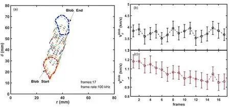
Figure 2.(a) Simultaneously recognizing a blob in 17 consecutive frames,(b) trajectory tracking exported blob poloidal velocity and (c)radial velocity.

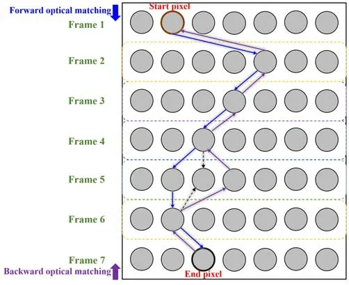
Figure 3.The improved method for forward and backward timing search process diagram.The bifurcation pixel between forward search and backward search in the Frame 5 makes the flow path be optimized.

2.3.Velocity field map

To further derive the velocity field,an improved technique akin to dense optical flow is employed to calculate the turbulent velocity field map within GPI data.This TDE technique is based on dense optical flow analysis to examine the positional changes of pixels between frames [22,23].An inverse time sequence search is introduced,which extracts the turbulent evolution displacement not only from forward to backward but also from backward to forward.

As illustrated in figure 3,the sequence comprises seven frames,and the movement trajectory of a specific pixel is obtained by conducting a forward or downward search.Simultaneously,a backward or upward search is performed from the end pixel to acquire another movement trajectory.In the event of inconsistency between the two trajectories,the track line is adjusted accordingly.After confirming that both vectors are within the turbulent boundary plasma,we add the two velocity vectors to obtain the new velocity vector.

The improved TDE technique operates on several key principles.The first step involves constructing a two-layer image pyramid to circumvent aperture issues [24].The technique defines an objective function to evaluate pixel displacement between frames.This objective function,G(d),is as follows:

Here,drepresents the displacement vector,is the matching cost function withPsymbolizing the patch set,and ω·L(d) is the regularization term.The matching cost function can be expanded as,

Here,qdenotes an offset vector within patchP,andT(P)signifies the patch following a discrete Fourier transform(DFT).I1represents the image gradient in the first frame,whileI2refers to the second frame.The regularization term,ω·L(d),ensures smoothness and consistency in the estimated motion field,with the total variation (TV) regularization term being used.L(d) can be written as:

where ω is set as a coefficient matrix correlated to the radial position of the SOL.The initial result,d,can be obtained by iteratively calculating the objective functionG(d).The initial search area is defined by a neighborhoodN(p)centered around the initial displacement vector estimationd.Ifd′symbolizes the updated displacement estimation at the initial pixel following the execution of the inverse search,d′should be written as:

They wandered in the woods the whole day, but could not find their way out. As night fell they found an inn and went inside. The servant gave the raven to the innkeeper to prepare for supper.

After iteratively updating the displacement field in this manner,the search can efficiently converge on a solution that minimizes the objective function.It should be noted that the blob contour area and non-blob one,extracted in section 2.2,belong to two distinct patch sets and only share pixels near the boundary.Thus,two different sets of parameters are employed to derive the velocity field map for the contour areas.

The improved TDE technique allows for the derivation of a velocity vector map from two frames separated by a time interval.Figures 4(a) and (b) illustrate the development of a coherent structure in the left region of the images,propagating in the SOL.Figure 4(c) presents a velocity quiver map calculated from figures 4(a) and (b) with the interval of 10μs.Each pixel velocities,vxandvy,are computed using the improved TDE technique.To make the figure clearer four adjacent velocity vectors are subsequently merged into one.In these frames,thevxof the middle plane is approximately 1 km s-1,and the poloidal velocityvyis about 4 km s-1.This aligns with both theoretical predictions and experimental observations of blob velocities [25-27].

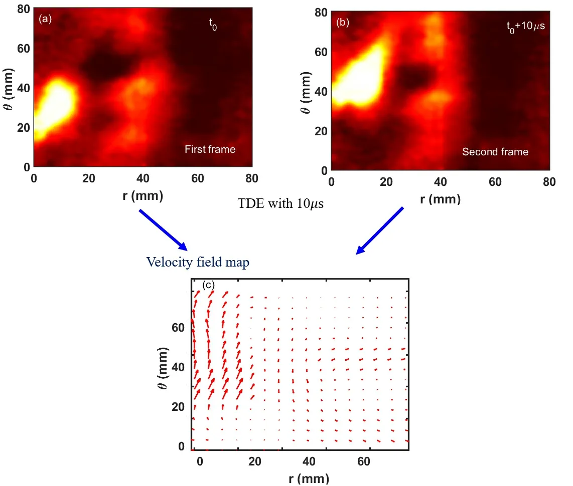
Figure 4.Contour plots of intensity at two successive times with the separation of 10 μs ((a) and (b)),and the derived velocity map with the TDE technique (c).

It is important to note that the original velocity vector units are pixels [25-27].Figure 4(c) clearly demonstrates the movement of the blob near the LCFS towards the first wall,where the length of the arrow represents relative velocity.The actual turbulence movement velocity can also be determined from the time delay between the two frames and the distance between pixels.

2.4.Comparison of standard TDE with improved one

We assessed the standard TDE algorithm and its enhanced variant by comparing their error rates,memory usage,and execution times.This comparison used GPI data from three discharges at a resolution of 256×256 pixels and a frequency of 100 kHz on the HL-2A tokamak.Both algorithms were executed in an identical virtual machine environment and to accurately measure the memory usage of both the standard and improved TDE algorithms during runtime,we employed a profiling tool that monitors the allocation and deallocation of memory in real time.This tool records the peak memory consumption,which represents the maximum amount of memory used by the program at any point during its execution.With each discharge comprising 400-500 images,we tabulated the average outcomes of the three discharges in table 1.

According to the data presented,the improved algorithm achieves a more substantial reduction in error compared to the standard algorithm,while only incurring a marginal increase in execution time.The slight rise in time required is negligible and within the processing capabilities of a stan-dard personal computer.Meanwhile,as shown in figure 5,we directly present a comparative illustration of the standard and the improved velocity field maps over time.Each velocity field map is spaced by 10μs,derived from four frames of data calculated pairwise consistent with the process illustrated in figure 4.Figure 5(a) represents that the results of the two methods are basically consistent.However,it is evident in figure 5(b),specifically in the upper right corner(within the purple dashed line),that the velocity vectors of the standard algorithm exhibit significant distortion.This distortion persists into the subsequent velocity field map diagram in figure 5(c).Apart from the above mentioned,the difference between the two methods is not significant during this period,but it is foreseeable that the error accumulated by a long time series will make the improved method have obvious advantages.Therefore,a direct comparison underscores the superiority of the improved method in terms of accuracy.

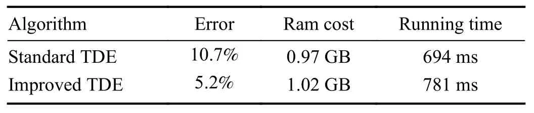
Table 1.Comparison of the standard TDE algorithm and the improved one.

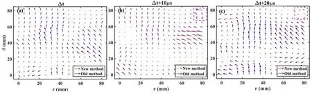
Figure 5.(a)-(c) Three successive velocity field maps provide a direct comparison between the improved algorithm (new method) and the standard algorithm (old method) based on calculations from four consecutive frames.

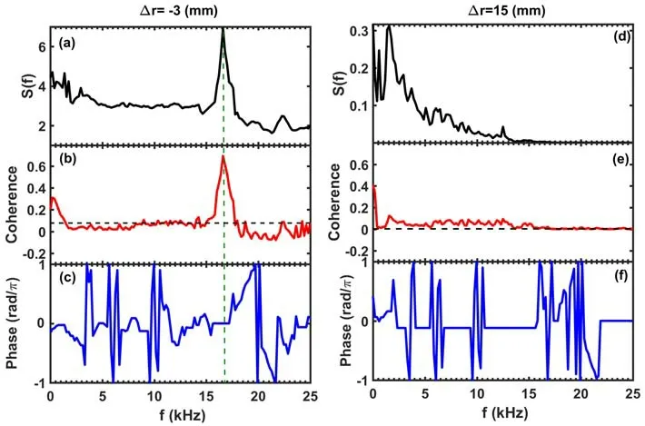
Figure 7.Contrasts of spectral cross-power (a),(d),the cross-coherence (b),(e) and phase (c),(f) at two radial positions estimated from two poloidal velocities with poloidal separation dθ ≈ 9 mm.

3.Experimental confirmation

The TDE technique is a valuable tool to analyze boundary plasma profiles.For example,when the TDE approach is applied to a series of images,a succession of velocity vectors in thexandydirections can be derived.By averaging the velocity direction ofxory,profiles of specific positions in the poloidal or radial direction can be obtained.

Figures 6(a)-(c) display radial profiles of poloidal velocityVθ,shear flow,and Reynolds stress,with theθdirection chosen near the middle plane.The dashed area represents the error bar,calculated by the standard deviation defined as ε(i)=Observations from figure 6 demonstrate that the radial profiles are notably different inside and outside the LCFS,with the rapid movement of blobs in SOL causing a ramp-up of parameters outside LCFS.Local poloidal velocities reach up to about -2km s-1(in the electron diamagnetic direction),and Reynolds stress is up to～ 4 × 106m2s-2(outward) inside LCFS.Since the velocity is directly calculated,its profiles obtained by improved TDE method are directly derived and comparable to those calculated by the Langmuir probes arrays in the SOL regions,with rather high reasonable.

This TDE technique can be extended for analyzing zonal flows and MHD-correlated blobs [16].To exemplify spectral analysis,the poloidal velocities,derived as single-channel signals,are further investigated using the two-point technique [28,29].Figures 7(a)-(f) contrast the spectral crosspower,cross coherence and phase using poloidal velocities at two radial positions of Δr=-3 mm and Δr=15 mm.A coherent mode peaking at 17 kHz with strong power and coherence of 0.8 is discernible in the spectrum at Δr=-3 mm.Short wavenumber components of the turbulence are filtered in the spectra due to the long distance between poloidal positions.

Interestingly,the cross-phase of the coherent mode frequency is almost zero,distinguishing it from the highfrequency parts of ambient turbulence,as shown in figure 7(c).In contrast,no similar correlation peak is observed at Δr=15 cm,with only the spectrum of turbulence being observed.This could potentially indicate the presence of coherent poloidal flow fluctuations at Δr=-3 mm,i.e.,the presence of geodesic acoustic modes (GAM).These results are consistent with the GAM characteristics observed in a tokamak [30,31].The results demonstrate that the improved TDE technique has the potential for analyzing GAM,MHDcorrelated blobs,and turbulence in the frequency domain.

4.Conclusion

An improved TDE technique presented in this study provides a comprehensive framework for detecting,tracking,and characterizing turbulence structures based on GPI data.It employs an inverse timing search,utilizes coarse-to-fine processing,and uses a hierarchical approach to improve calculation efficiency,accuracy,and robustness to noise.This technique is less susceptible to variations with light intensity in GPI data and better addresses large displacement issues.The proposed methods,including the application of the TDE technique and an improved optical flowbased approach,can effectively calculate and analyze turbulent velocity field maps and blob dynamics.The TDE technique can observe significant distinctions in the radial profiles inside and outside the LCFS and fast motion of blobs in the SOL.It is important to note that the improved TDE technique has a smaller error compared to the standard TDE technique,and the directly measured velocity field maps is comparable to the results of the Langmuir probe.The power spectral analysis reveals the possibility of identifying coherent modes and distinguishing them from ambient turbulence.The application of TDE technique extends beyond blob analysis,which shows the potential in examining zonal flows and MHD-correlated blobs.This TDE technique substantially improves the ability to study boundary plasma turbulence and transport related physics based on GPI data.Future research should focus on refining these techniques and exploring their applications in other related fields.It would provide a useful tool to analyze boundary plasma physics.Meanwhile,it may be applied to other plasma diagnostics.

Acknowledgments

This work is partially supported by the National Key R&D Program of China (Nos. 2019YFE03030002 and 2022YFE03030001),National Natural Science Foundation of China (Nos.12175186 and 12175055),and the Natural Science Foundation of Sichuan Province (Nos.2022NSFSC1820 and 2023NSFSC1289).