Design space exploration of neural network accelerator based on transfer learning①

WU Yuzhang(吴豫章), ZHI Tian②, SONG Xinkai, LI Xi

(∗School of Computer Science, University of Science and Technology of China, Hefei 230027, P.R.China)

(∗∗State Key Lab of Processors, Institute of Computing Technology, Chinese Academy of Sciences,Beijing 100190, P.R.China)

Abstract

Key words: design space exploration (DSE), transfer learning, neural network accelerator,multi-task learning

0 Introduction

Artificial intelligence (AI) algorithms, particularly deep neural networks, have demonstrated remarkable results in various fields such as image recognition and natural language processing.Initially, neural networks were executed on central processing unit(CPU), but with the development of the algorithms, it was discovered that graphics processing unit (GPU),with their parallel computing capabilities, were better suited for these calculations.To maintain computational efficiency while reducing power consumption, dedicated neural network accelerators such as Eyeriss[1],Google tensor processing unit (TPU)[2], Tesla neuralnetwork processing unit (NPU)[3], and others have been proposed.

As algorithmic advancements continue, the architecture of dedicated accelerators must be updated to accommodate these changes.Different accelerators have varying memory levels, data flow, and mapping of processing element (PE) arrays.To find a globally optimal solution rather than a local optimal solution, these configurations must be explored in the parameter space.Consequently, researchers are seeking ways to automate the design of neural network accelerators while accounting for constraints.In recent years, many studies have focused on the design automation of deep neural network (DNN) accelerators, including Dnn Weaver[4], DNNBuilder[5], AutoDNNchip[6], ConfuciuX[7], among others.

Design space exploration (DSE) plays a critical role in optimizing the performance and efficiency of neural network accelerators, which are specialized hardware devices designed to accelerate the computation of neural networks.DSE algorithms typically involve exploring a large number of possible parameter configurations, such as the number and type of processing elements (PEs), memory sizes, and interconnect architectures, to find the optimal set of parameters that meets certain design objectives, such as throughput, power consumption, or area.Different DSE tools and frameworks have been proposed to automate and optimize the process of exploring the design space, by using various techniques such as simulation, modeling,and machine learning.The work of DSE in recent years includes Interstellar[8], simulating machine learning applications using gem5-aladdin (SMAUG)[9], Accelergy[10], dMazeRunner[11], and loop-order-based memory allocation (LOMA)[12].These DSE tools have the potential to significantly reduce the design time and cost of neural network accelerators, and enable the design of highly customized and efficient hardware for specific neural network workloads.However, DSE also presents some challenges, such as the large search space, the complexity of the hardware design, and the need to balance multiple conflicting design objectives.

In this work,the extension of the concept of transfer learning to improve the performance of a target learning task by reusing knowledge from a related source task or domain is proposed.Unlike traditional machine learning algorithms, transfer learning has the advantage of reducing the training time of a pretrained model, which can be applied to similar processor architectures.The parameters abstracted by different processor architectures are reused, a part of the hidden layer of the pre-trained model is reserved, and the input hidden layer is retrained to adapt to the target task.

The similarities in the design space of different tasks performed by the unified intelligent processor architecture are explored.Transfer learning can use either hard parameter sharing or soft parameter sharing to optimize the shared model.Hard parameter sharing means that multiple tasks share a common model,while soft parameter sharing allows each task to have its own model and parameters, where some parameter values are shared among all tasks.To address the challenge of different input sizes, the use of hard parameter sharing to connect sub-model structures is proposed,where each task has its own sub-model.

The paper is organized as follows.In Section 1,the computing task on a neural network accelerator and how design parameters affect the latency and energy results are described.Section 2 is related work.Section 3 describes the proposed methodology for DSE based on transfer learning.In Section 4, experimental results demonstrate the effectiveness of the methodology are presented.The concluded and future research directions are discussed in Section 5.

1 Problem description

1.1 Convolutional neural networks (CNN)accelerator

The applications of CNN are numerous and cross many disciplines.They can be particularly useful in the fields of robot control, image identification, and natural language processing.CNN can help recognize items in photos and categorize them by using image recognition, it can recognize text and produce relevant outputs in natural language processing, and it can also aid robot navigation and object recognition in robot control.

CNN uses convolution operations to process input data.Convolution operation involves taking a small matrix, known as a kernel or filter, and sliding it over the input matrix to compute a new output matrix.

Fig.1 depicts the convolution operation, whereOstands for the output matrix,Ifor the input matrix,andWfor the convolution matrix;CIdenotes the number of input channels,COdenotes the number of output channels, andWOandHOdenote the width and height of the output tensor, respectively, andKWandKHdenote the width and height of the convolution kernel.

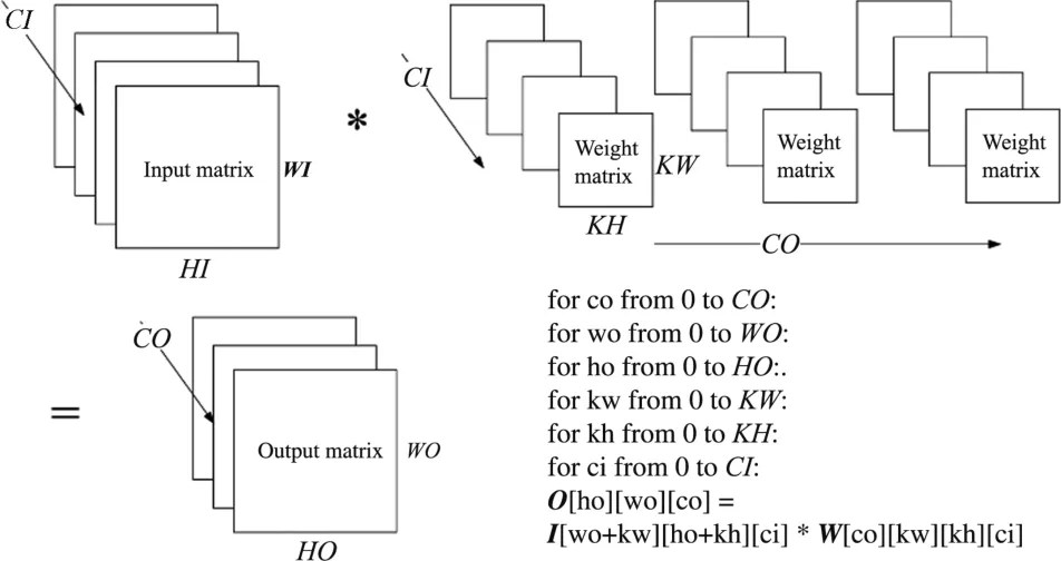
Fig.1 Convolutional computation written as a loop

A dedicated neural network accelerator is a hardware device specifically designed to accelerate convolution operations in deep neural networks.These accelerators leverage the parallelism inherent in convolution operations to perform them faster and more efficiently than general-purpose CPUs or GPUs.

The memory hierarchy in a neural network accelerator typically consists of several levels of memory as shown in Fig.2, ranging from on-chip registers and caches to off-chip dynamic random-access memory(DRAM).This hierarchy is designed to minimize memory access time and optimize data transfer between different levels of memory.

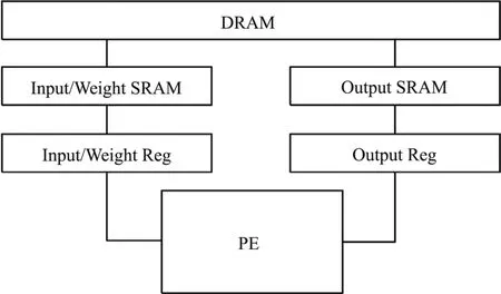
Fig.2 In a neural network accelerator, the PEs usually have dedicated registers that store intermediate results during computation

Design parameters in dedicated neural network accelerators involve various hardware-level optimizations to improve performance, energy efficiency, and accuracy.These parameters include the size of on-chip memory, the number and type of processing units, the dataflow and scheduling of computations, and the precision of data representation.The design parameters can significantly affect the performance and power consumption of the accelerator, as well as the accuracy of the neural network inference.Therefore, exploring the design space and identifying the optimal set of design parameters is crucial for achieving high-performance and energy-efficient neural network accelerators.

1.2 Spatial mapping and temporal mapping

The mappings determine the approach for executing the computation of a neural network on a hardware accelerator, and can be classified into two distinct types.

(1)Spatial mapping.The movement of operands across PE arrays in the spatial dimension is governed by spatial mappings.The selected mapping for a neural network computation on a hardware accelerator can greatly impact the level of data reuse per operand.As a result, the frequency of accessing storage outside the array can be reduced.

(2)Temporal mapping.Temporal mapping determines the order in which multiply-accumulate (MAC)operations are executed within each PE of every neural network layer.This is achieved by using a set of nested for loops that operate on the operands of the MAC operations, which are distributed across the memory hierarchy.Each loop is mapped to a specific memory level,such as different Static random-access memorys(SRAMs).The order, size, and layer dimension of the nested loops define the temporal map, which plays a critical role in maximizing data reuse and minimizing memory accesses.

Both spatial and temporal mappings are crucial considerations for optimizing hardware and software design in terms of their impact on DNN accelerator performance.Ultimately, the best mapping strategies will depend on the specific requirements of the DNN being accelerated, as well as the characteristics of the hardware and software being utilized.

The complete temporal and spatial mapping can be constructed based on the level and characteristics of the memory hierarchy that is provided.However,given that there are potentially millions to billions of uniform or uneven mappings in the very wide mapping space,evaluating each mapping point to determine the best one would be time-consuming (note that it is only mapping a neural network layer on a fixed architecture).To address this issue, a neural network model based on transfer learning is utilized to predict the architecture parameter space for the next iteration, thus reducing a significant amount of traversal work.

1.3 Pareto front in multi-objective optimization

The formal definition of the multi-objective optimization problem is as follows.

In above equations, the variablexdenotes the decision vector, whereNdenotes the number of independent variablesxi.fh(x) denotes the objective function,gj(x) denotes the equation constraint,hk(x)denotes the equation constraint, andH,J, andKrepresent their quantities, respectively.

Whenx1andx2meet the requirements,x1is said to dominatex2.For all objective purposes,x2is not worse thanx1.For at least one objective function,x1is strictly superior tox2.

The Pareto optimal solution set is the set of all possible undominated solutions, and the Pareto front is the boundary of the Pareto optimal solution set.The Pareto front is a useful tool for analyzing and visualizing the trade-offs between different objectives in these problems.

The concept of Pareto optimality is incorporated in this work to maintain an undominated solutions set during the search process.The main objective is to generate a set of solutions that are not dominated by any other solution in the search space in terms of multiple objective functions.

In each iteration of the algorithm, a new solution is generated and evaluated based on one or more objective functions that measure its performance.If the solution is not dominated by any of the solutions in the current set, it is added to the set, and the dominated solution is removed in the set.The Pareto front is used to guide the search process, which is a set of solutions that represent the optimal trade-off between different objectives as shown in Fig.3.

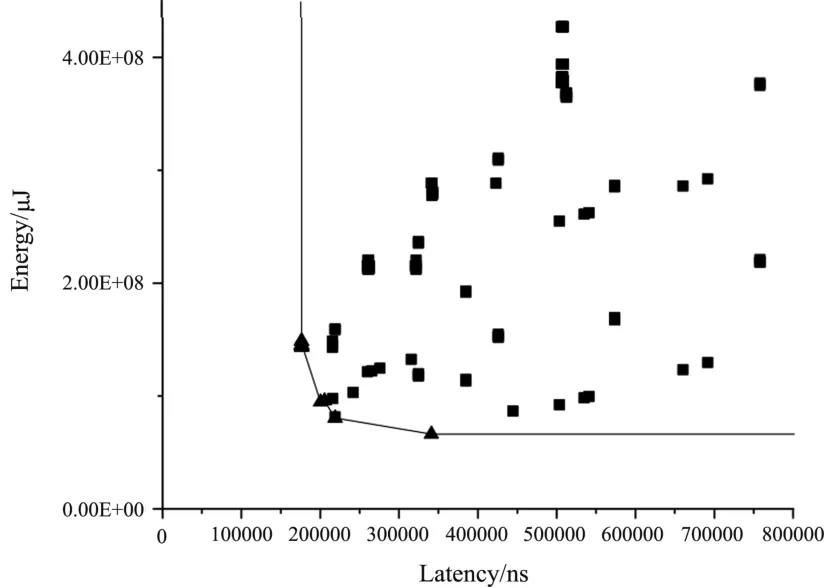
Fig.3 The scatter plot of latency and energy under different design parameters

It is possible that the search algorithm may not find a satisfactory result, meaning it may not converge to a single optimal solution.In such a scenario, the Pareto optimal solutions found during the search process can still be output.These solutions are considered non-dominated and represent the trade-off between the different objectives.Even though the search algorithm did not converge to a single optimal solution, the set of Pareto optimal solutions provides useful information to users on the best trade-offs between different objectives (energy, latency, and area).

1.4 DSE

DSE is a process of searching for an optimal set of architecture parameters and mapping parameters for a given set of computation tasks, subject to certain constraints.The goal is to find a design that optimizes a specific objective function, such as minimizing latency, maximizing throughput, or minimizing power consumption.

In this work, the input to the DSE process includes the architecture parameters, such as communication bandwidths, memory hierarchy, and interconnect topology, as well as the computation tasks, such as the data size, the number of operations, and the computational requirements of each task.The constraints may include resource limitations, power budgets, and timing requirements.

The DSE process involves exploring the design space to find the best architecture and mapping parameters that satisfy the constraints and optimize the objective function.The design space is defined by the possible values of the design and mapping parameters, and can be very large and complex.The search can be performed by using various techniques, such as bruteforce search, heuristic search, or optimization algorithms.

The output of the DSE process is a set of architecture parameters and mapping parameters that satisfy the constraints and optimize the objective function.The architecture parameters determine the hardware resources and organization, such as the number and size of processing elements, RAM sizes, and configurations.The mapping parameters determine how the computation tasks are mapped onto the hardware resources, such as the allocation of data to memory, the assignment of processing elements to tasks, and the scheduling of data transfers between the memory and the processing elements.

LetDdenotes the design parameters,Mdenotes the mapping parameters, andTdenotes the computational task.LetE(D,M,T) denotes the energy consumption of the accelerator with design parametersDand mapping parametersMand executing computational taskT.LetL(D,M,T) denotes the latency of the accelerator with design parametersD, mapping parametersMand executing computational taskT.

The goal of the design space exploration is to find the optimal set of design parameters and mapping parameters (D,M) that minimize the energy consumption and latency of the accelerator, subject to any constraints on the design parameters and mapping parameters.

This can be expressed as the following optimization problem.

whereDandMare the sets of valid design parameters and mapping parameters, respectively.

Solving this optimization problem requires exploring the design space by evaluating the energy consumption and latency for different combinations of design parameters and mapping parameters, and selecting the optimal set of parameters that satisfies the constraints and minimizes the objective function.This can be done by using various optimization techniques, such as simulated annealing(SA), heuristic search, or the proposed transfer learning-based approach.

2 Related work

Design space exploration is a critical step in optimizing the performance and efficiency of hardware accelerators for deep neural networks.However, exploring the design space can be time-consuming and computationally expensive.

Traditional methods, such as exhaustive search[13], random search[14], and SA[15], often require extensive search iterations to find the optimal design parameters and mapping parameters.This can result in long wait times and limited scalability, particularly when exploring complex design spaces.

To address this challenge, researchers have proposed several methods to accelerate design space exploration.Refs [16,17] introduced a fast approach for micro-architectural design space exploration and later improved the robustness of design space modeling.Chen et al.[18]explored the microprocessor design space by using unlabeled design configurations.Additionally, there are also some work exploring the design space of field programmable gate array (FPGA)-based accelerators, such as the design space exploration of FPGA accelerators for convolutional neural networks proposed by Rahman et al.[19]and the exploration of FPGA-based accelerators with multi-level parallelism presented by Zhong et al.[20].The proposed methods for micro architectural design space exploration may have limited applicability due to their focus on specific aspects of design optimization.

Zig-Zag[21]designed a mapping search engine by using heuristic search strategies to locate the optimal mapping points on energy and performance.Heuristics are problem-solving techniques that use practical methods to solve problems in a reasonable amount of time.In this case, mapping search engines use heuristics to guide the search towards more promising areas of the design space, rather than searching the entire space exhaustively.

AIRCHITECT[22]described a novel approach to design space exploration that involves using multilayer perceptron (MLP) to learn the optimization task and predict optimal parameters for custom architecture design and mapping space.This approach bypasses the iterative sampling of the design space using simulation or heuristic tools, which can be a costly process.

Confuciu X[7]leveraged the reinforcement learning (RL) method to guide the search process.The RL agent generates resource assignments as ‘actions’ that are evaluated by a fast analytical model for DNN accelerators called MAESTRO, and the environment outputs‘rewards’ that are used to train the underlying policy network.

3 Methodology

3.1 Overview

A novel approach based on transfer learning is proposed in this work to conduct design space exploration accurately and quickly as shown in Fig.4.The optimal design parameters and mapping parameters are predicted by utilizing an MLP based on previously learned experiences.Compared with traditional methods,using MLP can greatly reduce the number of iterations and can be accelerated by GPU.

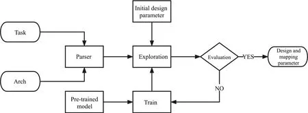
Fig.4 Flow chart for design space exploration

The design rationale for using transfer learning in this work is based on the principle that models trained on a particular task can be transferred to improve learning on a new,related task.By pre-training the MLP on a set of similar design problems,the learned knowledge can be used to guide the search process for a new problem.

Furthermore, it is demonstrated that the proposed method is superior to existing approaches that uses MLPs.MLP-based approaches require a large amount of data and are prone to overfitting, resulting in limited scalability and slower training times.In contrast, the transfer learning-based approach can use previously learned experiences to train the model,resulting in faster and more efficient training.

The algorithm is designed to provide optimal design and mapping parameters for a given processor architecture and computing task to achieve minimum power consumption and latency.It consists of four main phases: the parser phase, training phase, exploration phase, and evaluation phase.

In the parser phase, the input processor architecture and computing task information are translated into specific cycle scales, memory hierarchy, latency, and power consumption of different cell modules for further processing.

In the exploration phase, the algorithm generates candidate design parameter combinations to explore the design space.These combinations are either initialized at the start of the algorithm or updated based on the output of the neural network in the training phase.Once the candidate combinations are generated, the algorithm runs various mapping strategies in the simulator to calculate the latency and power consumption values for each combination.

In the training phase, a neural network model is trained and weighted based on the design and mapping parameters and their corresponding latency and power consumption.The neural network model is then used to make predictions, and the best candidate obtained is used as input for the next iteration of the exploration phase.

In the evaluation phase, the obtained candidate points are evaluated to determine whether the delay and power consumption meet the requirements.If the requirements are met, the design and mapping parameters are directly output.Otherwise, the algorithm enters the training phase.This process is iterated until the evaluation phase meets the exit criteria.

3.2 Parser phase

In the initial phase of the algorithm, the input accelerator architecture parameters are processed, including information on the memory structure from DRAM to PE, the optional calculation modes, and the power consumption and latency of each component during the calculation process.Based on this information, a processor object is instantiated in the simulator and the required design parameters can be determined.

Next, the layer information of the neural network is considered.This includes the size of the input and output matrix, the shape of the convolution kernel,step size, padding, dilation rates, and other relevant parameters.This information is then converted into a computational task in the form of a loop to facilitate later operation and evaluation.

3.3 Exploration phase

During the exploration phase, the accelerator parameters are initialized for the first run.This includes the size of each level of memory, the choice of computation mode, and other factors that depend on the given accelerator architecture.

The initialization of the accelerator parameters can be performed using a completely random initialization,or a pre-trained model can be used to estimate the optimal merit of the architecture based on the results of the previous design.

If it is not the first run, the candidate design parameter points can be obtained from the training phase,where the neural network has been trained on previous design parameters and mapping parameter combinations and their corresponding latency and power consumption results.Then a neural network can be used to predict the most advantageous design parameters combinations for the next iteration of the exploration phase.

Different mapping strategies are run in the simulator by using the initialized or candidate design parameters.Each mapping strategy generates a set of mapping parameters combinations and their corresponding latency and power consumption results.The mapping parameters combinations are the parameters used to map the computation onto the hardware accelerator, such as the choice of loop unrolling factors, tiling factors, and parallelization factors.

Once the mapping strategies are executed, the algorithm evaluates the results and selects the mapping parameters combination with the optimal latency and power consumption.Then the mapping parameters combination is used as input for the training phase.The exploration phase continues until the exit criteria are met, such as achieving the desired latency and power consumption targets or reaching a maximum number of iterations.

3.4 Training phase

In order to anticipate the optimum performance and power consumption for the optimal mapping case in architectures with various design parameters, a transfer learning model is trained.

The neural network model consists of seven fully connected layers.The input layer will determine the width of the input according to the design parameters required by the accelerator architecture obtained in the parser stage, and the output layer will output the latency and energy corresponding to the architecture parameters.

Before the training process starts, the 1st, 2nd,6th, 7th and 8th layers need to be randomly initialized, and after pruning and fine-tuning the weights of pre-trained models trained under other architectures,they are applied to the 3rd, 4th, and 5th layers as shown in Fig.5.

Fig.5 The transfer learning neural network structure consists of various layers that accept design parameters and task information as input and output corresponding energy and latency

Pruning and fine-tuning can improve the performance of the pre-trained model on the new task while reducing the amount of new data needed for training.By removing unimportant or redundant parameters through pruning, the model becomes more efficient and easier to train.Fine-tuning allows the pre-trained model to be adapted to the new task by adjusting its existing weights and biases to fit the new data, which can lead to better performance on the new task.A method similar to PAC-Net[23]is used.

Supposefws:X→Yis a model trained on the source data set, its weight vector isws, using minimizing the standard negative log-likelihood method for fine-tuning the pre-training model.

Then, for the weight vectorw= (w1,w2,...,wN) , the maskm= (m1,m2,...,mN) is used to remove smaller weights.

wherewtis a manually set threshold.

Next, the remaining unpruned vectors are embedded with the remaining information, which is represented aswU=w☉m.

Finally, adjust the pruned vectorwP=w☉(1 -m).

The target weight vectorfwtis obtained by addingwuandwP.

Since it is a multi-objective optimization, the loss function needs to use a balanced loss function:

whereNrepresents the total number of samples,enirepresents the predicted energy of thei-th sample,en︿irepresents the actual energy of thei-th sample, andlairepresents thei-th sample.The predicted latency of theisample,la︿irepresents the actual latency of thei-th sample, because the magnitude of the two is different,so the weightαneeds to be set.

According to the results of the exploration phase,substitute the accelerator parameters and optimal delay power data of this iteration into the model for training,and adjust the transfer learning model network weights.Then use the network to predict the energy and latency of other points, so as to select the next batch of candidate parameters for the optimal solution.This iteration is repeated until the evaluation phase is successfully completed.

3.5 Evaluation phase

In this phase, it is determined whether the search process can be terminated by judging whether the output satisfies a predetermined threshold for latency and power consumption.

If both energy and latency are less than the target:

the search can be ended immediately.

However, this situation is difficult to obtain directly during training, so it cannot be used to evaluate the quality of results.The following formula is used for comparison:

If results that simultaneously meet the objectives have not been achieved, the number of iterations can be set to force the algorithm to stop and output the result with the highest Qor achieved until that iteration.

4 Experiments

4.1 Overview

In this article, the experiment uses Python, taking AlexNet, VGG, and other networks as benchmarks to explore the design parameters of Google TPU, Eyeriss, and Tesla prototype architectures, the design parameters are shown in Table 1.The running example decomposes the network into layer-by-layer convolution or vector operations.Taking AlexNet as an example,the main computing tasks include different convolutional layers.

Table 1 The design parameters

4.2 Comparison with other methods

To assess the effectiveness of this method, several other methods are selected and modified to enable a fair comparison.These methods are as follows.

SA: SA is used as a baseline comparison method.SA iteratively explores the design space by making random modifications to the current architecture, accepting or rejecting changes based on a probability distribution dependent on the current temperature.The temperature decreases over time, becoming more restrictive and allowing the algorithm to converge towards a minimum.The initial temperature is set as 2 ×10-8.

Deep reinforcement learning (DRL): the policy gradient approach is used in the DRL method, similar to ConfuciuX[7].An actor network is used to update the policy network, with the current network parameters and configurations as states and modifications to the configurations as actions.Rewards are obtained when the current action approaches the states that satisfy the objectives, with a bonus added if the current state already satisfies the objectives.Hyper parameter tuning is performed to obtain relatively better results.

Large multilayer perceptron (Large MLP): the results were tested by applying MLP alone, similar to AIRCHITECT[22], and by applying the design selector to improve the results.AlexNet was run on the Google TPU architecture, and energy and latency were predicted based on the design parameters, withk-fold crossvalidation used for training.Once training is complete,a new training task is performed on Eyeriss architecture to run VGG16, and the randomly initialized network is compared with the network that had transferred the previous training results.As shown in Fig.6, the training efficiency of the transfer network is significantly improved.

Fig.6 The training losses of the transfer learning model and the MLP model without transfer learning

Heuristic method: similar to Zig-Zag[21], this is a DSE algorithm that iteratively searches for promising designs and refines them.The algorithm takes advantage of the fact that a design can often be decomposed into a set of sub-designs, each of which can be optimized independently.An optimal solution can be eventually converted by iteratively refining these sub-designs.

The transfer learning method is evaluated by running different convolutional network layers ten times using different methods, allowing a margin of error of 1%for the resulting delay and power measurements.This means that if the latency and power of the DSE output are not worse than the user’s target, the target is still considered satisfied.

The starting point of design space exploration are randomly initialized before the start of the DSE algorithms, and different DSE algorithms are running until they meet the conditions or the number of iterations reaches the upper limit.The total running time of 10 independent runs is then counted,and the average iterations and number of satisfied results are displayed in Table 2, source model trained on Google-TPU-like architecture, CONV 1 -3 running on Eyeriss-like architecture, CONV 4 -6 running on Tesla-NPU-like architecture, CONV 7 - 9 running on Meta-prototype-like architecture.These methods are run 10 times on 9 cases, for a total of 90 times, and count the number of the final output results of the algorithm that satisfy the requirements.The efficiency of different algorithms is compared by comparing the total time to obtain a result under a given constraint against a baseline of SA algorithm, as shown in Fig.7.The effectiveness of the transfer learning method is demonstrated by the comparisons made with other DSE methods.

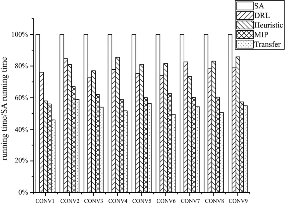
Fig.7 Comparison of runtimes of different DSE methods

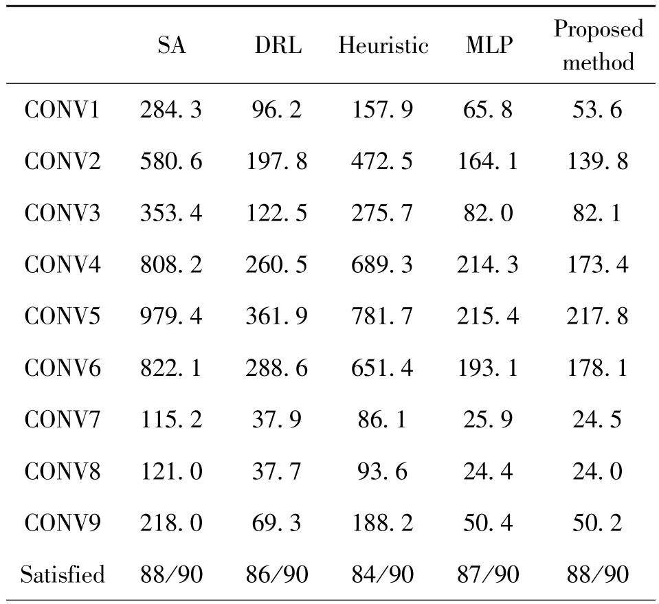
Table 2 Average iterations of different methods

4.3 Multi-task learning

Multiple tasks need to be handled by an accelerator, so the situation of exploring multiple tasks simultaneously needs to be considered.Three different scenarios are compared in this study.

Repeat: the DSE framework can be run repeatedly for a variety of different inputs to obtain the optimal parameter configuration under their respective conditions.The biggest advantage of this method is that it does not need to change any framework and input.

Merge: the approach is to merge the computing tasks of multiple problems into a single problem, which increases the time per iteration but reduces the number of iterations required.This results in a significant improvement in the method’s operating efficiency compared with repeated operations.Although there may be inconsistencies in the length of input parameters, the solution is to simply expand the input width.

Multi-task: to simultaneously evaluate the performance of multiple tasks, a multi-task model based on transfer learning is employed.To enable the model to process different tasks simultaneously, the transfer learning model is modified as shown in Fig.8.Specifically, an independent 1st layer is created for each input, with no interference between the 1st layers of different tasks.This approach addresses the issue of different numbers of input parameters between different tasks.Layers 2 -6 remain the same as described in Section 3,with the 2nd and 6th layers randomly initialized and the 3rd, 4th, and 5th layers transferred from the pre-trained model.The 7th and 8th layers are also divided into independent modules, each corresponding to the output of a different task.

Fig.8 The structure of transfer learning model in different tasks

The efficiency of the three proposed scenarios is evaluated by conducting multiple runs of the DSE algorithm using each scheme with different test sets, and the algorithm is terminated once the performance goal is achieved.Specifically, the final results had to meet the performance goal.Ten independent runs are conducted for each scenario and the average performance is calculated, as illustrated in Fig.9.The results demonstrate that the multi-task model outperforms the repeat model and is marginally superior to the merge model.The multi-task model significantly improves efficiency and enables a more comprehensive analysis of design space.

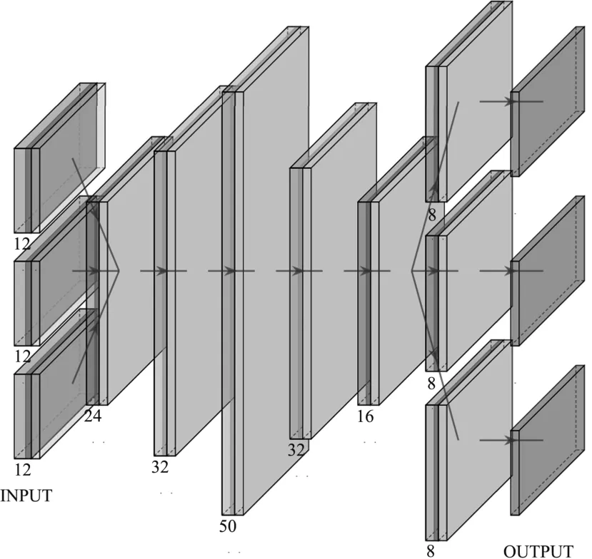
Fig.9 Comparison of DSE times using different methods in multi-tasking scenarios

5 Conclusion

In this study, a new DSE method is proposed for neural network accelerator design based on transfer learning.A new approach is presented that can accurately predict energy and latency performance parameters using neural networks that can learn from various accelerator architectures and tasks.Compared with other DSE tools,higher operating efficiency is achieved by this method.Furthermore, improved performance is achieved through the multi-task learning model, which allows simultaneous evaluation of multiple neural networks run samples in design space exploration.The framework is not limited to the simplified model used in this study, it can also be applied to more complex models, such as cycle-accurate electronic system level(ESL) simulators, to explore design spaces.Future work will focus on extending the scope of the framework to various simulators.