A Lyapunov characterization of robust policy optimization

Leilei Cui·Zhong-Ping Jiang

Abstract In this paper,we study the robustness property of policy optimization(particularly Gauss–Newton gradient descent algorithm which is equivalent to the policy iteration in reinforcement learning)subject to noise at each iteration.By invoking the concept of input-to-state stability and utilizing Lyapunov’s direct method,it is shown that,if the noise is sufficiently small,the policy iteration algorithm converges to a small neighborhood of the optimal solution even in the presence of noise at each iteration.Explicit expressions of the upperbound on the noise and the size of the neighborhood to which the policies ultimately converge are provided.Based on Willems’fundamental lemma,a learning-based policy iteration algorithm is proposed.The persistent excitation condition can be readily guaranteed by checking the rank of the Hankel matrix related to an exploration signal.The robustness of the learning-based policy iteration to measurement noise and unknown system disturbances is theoretically demonstrated by the input-to-state stability of the policy iteration.Several numerical simulations are conducted to demonstrate the efficacy of the proposed method.

Keywords Policy optimization·Policy iteration(PI)·Input-to-state stability(ISS)·Lyapunov’s direct method

1 Introduction

Through reinforcement learning(RL)techniques,agents can iteratively minimize the specific cost function by interacting continuously with unknown environment.Policy optimization is fundamental for the development of RL algorithms as introduced in[1].Policy optimization first parameterizes the control policy,and then,the performance of the control policy is iteratively improved by updating the parameters along the gradient descent direction of the given cost function.Since the linear quadratic regulator (LQR)problem is tractable and widely applied in many engineering fields, it provides an ideal benchmark example for the theoretical analysis of policy optimization.For the LQR problem, the control policy is parameterized by a control gain matrix,and the gradient of the quadratic cost with respect to the control gain is associated with a Lyapunov matrix equation.Based on these results, various policy optimization algorithms, including vanilla gradient descent, natural gradient descent and Gauss–Newton methods,are developed in[2–5].Compared with other policy optimization algorithms with a linear convergence rate,the control policies generated by the Gauss–Newton method converge quadratically to the optimal solution.

It is noticed that the Gauss–Newton method with the step size of 1/2 coincides with the policy iteration(PI)algorithm[6, 7], which is an important iterative algorithm in RL and adaptive/approximate dynamic programming (ADP) [1, 8,9].From the perspective of the PI, the Lyapunov matrix equation for computing the gradient can be considered as policy evaluation.The update of the policy along the gradient direction can be interpreted as policy improvement.The steps of policy evaluation and policy improvement are iterated in turn to find the optimal solution of LQR.Various PI algorithms have been proposed for important classes of linear/nonlinear/time-delay/time-varying systems for optimal stabilization and output tracking [10–14].In addition,PI has been successfully applied to sensory motor control[15],and autonomous driving[16,17].

The convergence of the PI algorithm is ensured under the assumption that the accurate knowledge of system model is accessible.However, in reality, the system model obtained by system identification [18] is used for the PI algorithm or the PI algorithm is directly implemented through a data-driven approach using input-state data [10, 19–22].Consequently,the PI algorithm is hardly implemented accurately due to modeling errors, inaccurate state estimation,measurement noise,and unknown system disturbances.The robustness of the PI algorithm to unavoidable noise is an important property to be investigated, which lays a foundation for better understanding RL algorithms.There are several challenges for studying the robustness of the PI algorithm.Firstly, the nonlinearity of the PI algorithm makes it hard to analyze the convergence property.Secondly, it is difficult to quantify the influence of noise,since noise may destroy the monotonic property of the PI algorithm or even result in a destabilizing controller.

In this paper,we study the robustness of the PI algorithm in the presence of noise.The contributions are summarized as follows.Firstly,by viewing the PI algorithm as a nonlinear system and invoking the concept of input-to-state stability(ISS)[23],particularlythesmall-disturbanceISS[24,25],we investigate the robustness of the PI algorithm under the influence of noise.It is demonstrated that when subject to noise,thecontrolpoliciesgeneratedbythePIalgorithmwilleventually converge to a small neighborhood of the optimal solution of LQR as long as noise is sufficiently small.Different from[24,25],where the analysis is trajectory-based,we directly utilize Lypuanov’s direct method to analyze the convergence of the PI algorithm under disturbances.As a result,an explicit expression of the upperbound on the noise is provided.The size of the neighborhood in which the control policies will ultimately stay is demonstrated as a quadratic function of the noise.Secondly,by utilizing Willems’fundamental lemma,a learning-based PI algorithm is proposed.Compared with the conventional learning-based control approach where the exploratory control input is hard to design such that the persistent excitation condition is satisfied[24],the persistently exciting exploratory signal of the proposed method can be easily designed by checking the rank condition of a Hankel matrix related to the exploration signal.Finally, based on the small-disturbance ISS property of the PI algorithm, we demonstrated that the proposed learning-based PI algorithm is robust to the state measurement noise and unknown system disturbances.

The remaining contents of the paper are organized as follows.Section 2 reviews the LQR problem and the celebrated PI algorithm.In Sect.3,the small-disturbance ISS property of the PI algorithm is studied.Section 4 proposes a learningbased PI algorithm and the robustness of the algorithm is analyzed.Several numerical examples are given in Sect.5,followed by some concluding remarks in Sect.6.

2 Preliminaries and problem formulation

2.1 Policy iteration for discrete-time LQR

The discrete-time linear time-invariant(LTI)system is represented as

wherexk∈Rnanduk∈Rmare the state and control input,respectively;AandBare system matrices with compatible dimensions.

Assumption 1 The pair(A,B)is controllable.

Under Assumption 1,the discrete-time LQR is to minimize the following accumulative quadratic cost

whereQ=QT≻0 andR=RT≻0.The optimal controller of the discrete-time LQR is

whereV∗=(V∗)T≻0 is the unique solution to the following discrete-time algebratic Riccati equation(ARE)

For a stabilizing control gainL∈ Rm×n, the corresponding cost in (2) isJd(x0,-Lx) =, whereVL=(VL)T≻0 is the unique solution of the following Lyapunov equation

and the functionG(·):Sn→Sn+mis defined as

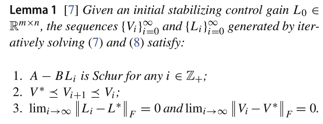
The discrete-time PI algorithm was developed by [7] to iteratively solve the discrete-time LQR problem.Given an initial stabilizing control gainL0,the discrete-time PI algorithm is represented as:

Procedure 1 (Exact PI for discrete-time LQR)

1.Policy evaluation:get G(Vi)by solving

2.Policy improvement:get the improved policy by

The monotonic convergence property of the discrete-time PI is shown in the following lemma.

2.2 Policy iteration for continuous-time LQR

Consider the continuous-time LTI system

wherex(t)∈Rnis the state;u(t)∈Rmis the control input;x0is the initial state;AandBare constant matrices with compatible dimensions.The cost of system(9)is

Under Assumption 1, the classical continuous-time LQR aims at computing the optimal control policy as a function of the current state such thatJc(x0,u) is minimized.The optimal control policy is

whereP∗=(P∗)T≻ 0 is the unique solution of the continuous-time ARE[26]:

For a stabilizing control gainK∈ Rm×n, the corresponding cost in (10) is, wherePK=(PK)T≻0 is the unique solution of the following Lyapunov equation

and the functionM(·):Sn→Sn+mis defined as

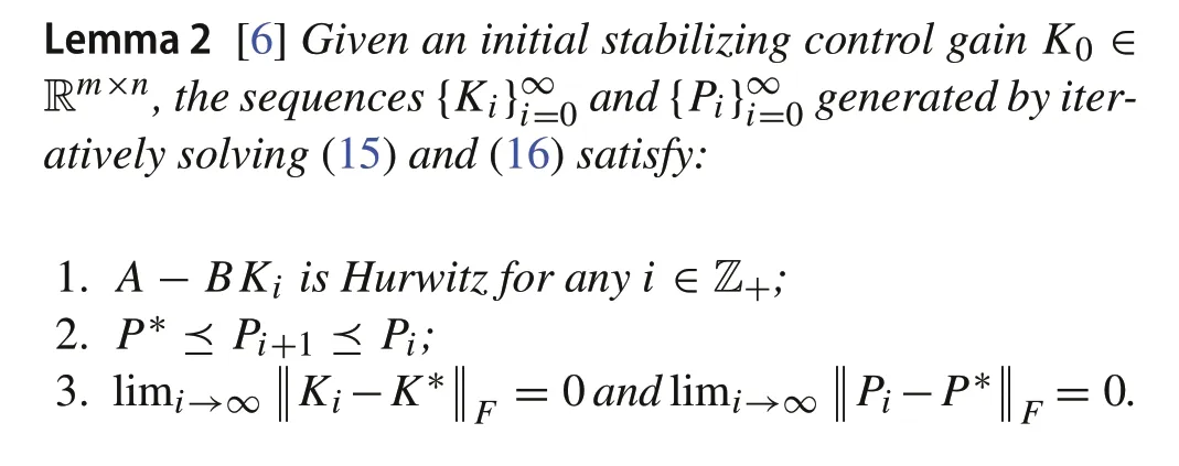
Given an initial stabilizing control gainK0, the celebrated continuous-time PI developed in[6]iteratively solves the continuous-time LQR problem.The continuous-time PI algorithm is represented as:

Procedure 2 (Exact PI for continuous-time LQR)

1.Policy evaluation:get M(Pi)by solving

2.Policy improvement:get the improved policy by

Given an initial stabilizing control gainK0,by iteratively solving(15)and(16),Pimonotonically converges toP∗and(A-BKi) is Hurwitz, which is formally presented in the following lemma.

2.3 Problem formulation

For the discrete-time and continuous-time PI algorithms,the accurate model knowledge(A,B) is required for the algorithm implementation.The convergence of the PI algorithms in Lemmas 1 and 2 are based on the assumption that the accurate system model is attainable.However,in reality,system uncertainties are unavoidable,and the PI algorithms cannot be implemented exactly.Therefore,in this paper,we investigate the following problem.

Problem 1When the policy evaluation and improvement steps of the PI algorithms are subject to noise,will the convergence properties in Lemmas1and2still hold?

3 Robustness analysis of policy iteration

In this section, we will formally introduce the inexact PI algorithms for the discrete-time and continuous-time LQR in the presence of noise.By invoking the concept of input-tostate stability[23],it is rigorously shown that the optimized control policies converge to a neighborhood of the optimal control policy,and the size of the neighborhood depends on the magnitude of the noise.

3.1 Robustness analysis of discrete-time policy iteration

According to the exact discrete-time PI algorithm in(7)and(8), in the presence of noise, the steps of policy evaluation and policy improvement cannot be implemented accurately,and the inexact PI algorithm is as follows.

Procedure 3 (Inexact PI for discrete-time LQR)

1.Inexact policy evaluation:getˆGi∈Sm+n as an approximation of G(ˆVi),whereˆVi is the solution of

2.Inexact policy improvement:get the improved policy by

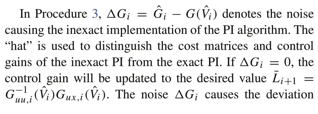
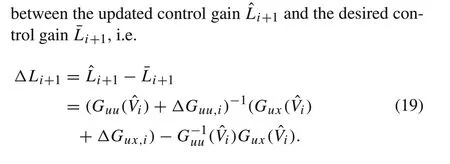
Remark 1The noiseΔGican be caused by various factors.For example, in data-driven control [24], the matrixG(ˆVi)is identified by the collected input-state data.Since noise possibly pollutes the collected data, ˆGi, instead ofG(ˆVi),is obtained.Other factors that may causeΔGiinclude the inaccurate system identification,the residual error of numerically solving the Lyapunov equation, and the approximate values ofQandRin inverse optimal control in the absence of the exact knowledge of the cost function.

Next,by considering the inexact PI as a nonlinear dynamical system with the state ˆVi, we analyze its robustness to noiseΔGiby Lyapunov’s direct method and in the sense of small-disturbance ISS.For any stabilizing control gainL,define the candidate Lyapunov function as

whereVL=≻0 is the solution of(5).SinceVL≥V∗(obtained by Lemma 1),we have

Remark 2SinceJd(x0,-Lx) =xT0VLx0, whenx0∼N(0,In),Ex0Jd(x0,-Lx)=Tr(VL).Hence,the candidate Lyapunov function in (20) can be considered as the difference between the value function of the controlleru(x(t))=-Lx(t)and the optimal value function.

For anyh> 0, define a sublevel setLh= {L∈Rm×n|(A-BL)is Schur,Vd(VL) ≤h}.SinceVLis continuous with respect to the stabilizing control gainL, it readily follows thatLhis compact.Before the main theorem about the robustness of Procedure 3, we introduce the following instrumental lemma,which provides an upperbound onVd(VL).

Lemma 3For any stabilizing control gain L,let L′=(R+BTVL B)-1BTVL A and EL=(L′-L)T(R+BTVL B)(L′-L).Then,

where

ProofWe can rewrite(4)as

It was the day before Thanksgiving -- the first one my three children and I would be spending without their father, who had left several months before. Now the two older children were very sick with the flu, and the eldest1 had just been prescribed bed rest for a week.

In addition,it follows from(5)that

Subtracting(24)from(25)yields

Since(A-BL∗) is Schur, it follows from [27, Theorem 5.D6]that

Taking the trace of(27)and using the main result of[28],we have

Hence,the proof is completed.■

Lemma 4For any L∈Lh,

ProofSince(A-BL)is Schur,it follows from(5)and[27,Theorem 5.D6]that

Hence,(29)readily follows from(31).■

The following lemma shows that the sublevel setLhis invariant as long as the noiseΔLiis sufficiently small.

ProofInduction is applied to prove the statement.Wheni=0, ˆL0∈Lh.Suppose ˆLi∈Lh,then,by[27,Theorem 5.D6],we have ˆVi≻0.We can rewrite(17)as

Considering(19),we have

In addition,it follows from(19)that

Plugging(33)and(34)into(32),and completing the squares,we have

where

If

it is guaranteed that

Writingdown(17)atthe(i+1)thiteration,andsubtracting it from(35),we have

Following[27,Theorem 5.D6],we have

Taking the trace of(40),and using Lemma 3 and the result in[28]yield

It follows from(41),Lemma 4 and[28]that

whereb2is defined as

Hence,if

it is guaranteed that

Now,by Lypaunov’s direct method and by viewing Procedure 3 as a discrete-time nonlinear system with the state ˆVi, it is shown that ˆViconverges to a small neighbourhood of the optimal solution as long as noise is sufficiently small.

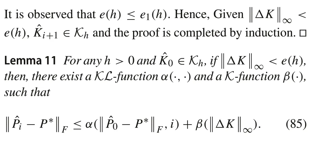
Lemma 6For any h> 0andˆL0∈Lh,if

there exist a K-function ρ(·)and a KL-function κ(·,·),such that

ProofRepeating(42)fori,i-1,...,0,we have

Considering(21),it follows that

The proof is thus completed.■

The small-disturbance ISS property of the Procedure 3 is shown in the following theorem.

Consequently,

3.2 Robustness analysis of continuous-time policy iteration

According to the exact PI for continuous-time LQR in(15) and (16), in the presence of noise, the steps of policy evaluation and policy improvement cannot be implemented accurately,and the inexact PI is as follows.

Procedure 4 (Inexact PI for continuous-time LQR)

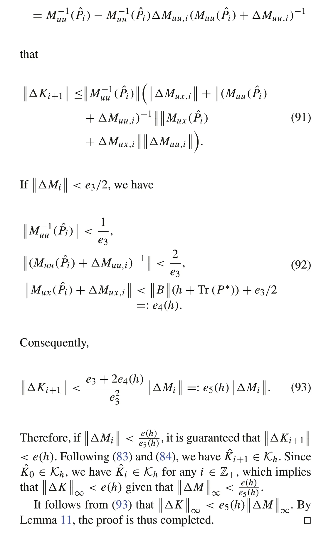
1.Inexact policy evaluation:getˆMi∈Sm+n as an approximation of M( ˆPi),whereˆPi is the solution of

2.Inexact policy improvement:get the updated control gain by

For any stabilizing control gainK, define the candidate Lyapunov function as

wherePK=≻0 is the solution of(13),i.e.

SincePK≥P∗,we have

Foranyh>0,definethesublevelsetKh={K∈Rm×n|(ABK)is Hurwitz,Vc(PK)≤h}.SincePKis continuous with respect to the stabilizing control gainK,the sublevel setKhis compact.

The following lemmas are instrumental for the proof of the main theorem.

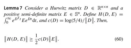
ProofThe Taylor expansion ofeDtis

Hence,

Pick av∈Rnwhich satisfies.Then,

Hence,the lemma follows readily from(63).■

The following lemma presents an upperbound of the Lyapunov functionVc(PK).

Lemma 8For any stabilizing control gain K,let K′=R-1BTPK,where PK=PTK≻0is the solution of(58),and EK=(K′-K)TR(K′-K).Then,

ProofRewrite ARE(12)as

Furthermore,(58)is rewritten as

Subtracting(65)from(66)yields

ConsideringK′=R-1BTPKand completing the squares in(67),we have

Since(A-BK∗) is Hurwitz, by (68) and [27, equation(5.18)],we have

Taking the trace of (69), considering the cyclic property of trace and[28],we have(64).■

Lemma 9For any K∈Kh,

ProofSinceA-BKis Hurwitz,it follows from(58)that

Taking the trace of(71),and considering[28],we have

The proof is hence completed.■

Writing down(54)for the(i+1)th iteration,and subtracting it from(75),we have

Since(A-BˆKi+1) is Hurwitz (e(h) ≤e1(h)), it follows from[27,equation(5.18)]and(78)that

Taking the trace of(79),and considering[28]and Lemma 9,we have

It follows from(80)and Lemmas 7 and 8 that

Taking the expression of ˆKi+1into consideration,we have

Plugging(82)into(81),it follows that if

we have

ProofIt follows from Lemma 10,(81)and(82)that for anyi∈Z+,

Repeating(86)fori,i-1,...,1,0,we have

By(59),we have

Hence,(85)follows readily.■

With the aforementioned lemmas, we are ready to propose the main result on the robustness of the inexact PI for continuous-time LQR.

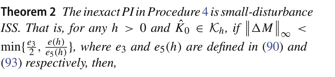
ProofSuppose ˆKi∈Lh.If

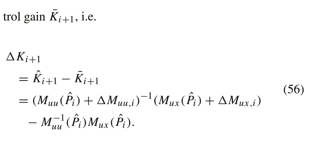
(ΔMuu,i+Muu( ˆPi))is invertible.It follows from(56)and

Remark 3Compared with[24,25],in Theorems 1 and 2,the explicit expressions of the upperbounds on the small disturbance are given, such that at each iteration, the generated control gain is stabilizing and contained in the sublevel setsLhandKh.In addition, it is observed from (48) and (88)that the control gains generated by the inexact PI algorithms ultimately converge to a neighborhood of the optimal solution,and the size of the neighborhood is proportional to the quadratic form of the noise.

4 Learning-based policy iteration

In this section,based on the robustness property of the inexact PI in Procedure 3,we will develop a learning-based PI algorithm.Only the input-state trajectory data measured from the system is required for the algorithm.

4.1 Algorithm development

For a signalu[0,N-1]= [u0,u1,...,uN-1], its Hankel matrix of depthlis represented as

Definition 1 An input signalu[0,N-1]is persistent exciting(PE)of orderlif the Hankel matrixHl(u[0,N-1])is full row rank.

Lemma 12 [31]Let an input signal u[0,N-1]be PE of order l+n.Then,the state trajectory x[0,N-1]sampled from system(1)driven by the input u[0,N-1]satisfies

Given the input-state datau[0,N-1]andx[0,N]sampled from (1), we will design a learning-based PI algorithm such that the accurate knowledge of system matrices is not required.For any time indices 0 ≤k1,k2≤N- 1 andV∈Sn,along the state trajectory of(1),we have

It follows from(96)that

Assumption 2 The exploration signalu[0,N-1]is PE of ordern+1.

Under Assumption 2 and according to Lemma 12,z[0,N-1]is full row rank.As a result,for any fixedV∈Sn,(98)admits a unique solution

whereΛis a data-dependent matrix defined as

Therefore, given anyV∈Sn,Θ(V) can be directly computed from(99)without knowing the system matricesAandB.

By(97),we can rewrite(7)as

Plugging(99)into(101)yields(102).The learning-based PI is represented in the following procedure.

Procedure 5 (Learning-based PI for discrete-time LQR)

1.Learning-based policy evaluation

2.Learning-based policy improvement

It should be noticed that due to(99),Procedure 5 is equivalent to Procedure 1.

4.2 Robustness analysis

In the previous subsection,we assume that the accurate data from system can be obtained.In reality,measurement noise and unknown system disturbance are inevitable.Therefore,the input-state data is sampled from the following linear system with unknown system disturbance and measurement noise

wherewk∼N(0,Σw)andvk∼N(0,Σv)are independent and identically distributed random noises.Let ˇzk=[yTk,uTk]and suppose there are in totalStrajectories of system(104)which start from the same initial state and are driven by the sameexplorationinputu[0,N-1].Averagingthecollecteddata overStrajectories,we have

Then,the data-dependent matrix is constructed as

By the strong law of large numbers,the following limitations hold almost surely

Recall thatz[0,N-1],x[1,N-1], andΛare the data collected from system (1) with the same initial state and exploration input as (104).SinceSis finite, the difference betweenΛand ˇΛSis unavoidable,and hence,

Procedure 6 (Learning-based PI using noisy data)

1.Learning-based policy evaluation using noisy data

2.Learning-based policy improvement using noisy data

In Procedure 6,the symbol“check”is used to denote the variables for the learning-based PI using noisy data.In addition,let ˜Videnote the result of the accurate evaluation of ˇLi,i.e.˜Viis the solution of(109)with ˇΘ(ˇVi)replaced byΘ(˜Vi).ˇVi= ˜Vi+ΔViis the solution of(109)andΔViis the policy evaluation error induced by the noiseΔΛ.In the following contents,the superscriptSis omitted to simplify the notation.Based on the robustness analysis in the previous section,we will analyze the robustness of the learning-based PI to the noiseΔΛ.

For any stabilizing control gainL,let ˇVL=VL+ΔVbe the solution of the learning-based policy evaluation with the noisy data-dependent matrix ˇΛ,i.e.

The following lemma guarantees that(111)has a unique solution(VL+ΔV)=(VL+ΔV)T≻0.

Lemma 13If

then(Λ+ΔΛ)TIn-LTTis a Schur matrix.

ProofRecall thatVL=VTL≻0 is the solution of(5)associated with the stabilizing control gainL.By (99), (5) is equivalent to the following equation

SinceQ≻0,by[30,Lemma 3.9],ΛTIn-LTTis Schur.

WhenΛis disturbed byΔΛ,we can rewrite(113)as

When(112)holds,we haveBy [30, Lemma 3.9], (114) and (115),(Λ+ΔΛ)T×In-LTTis Schur.■

The following lemma implies that the policy evaluation errorΔVis small as long asΔΛis sufficiently small.

Lemma 14For any h>0,L∈Lh,and ΔΛ satisfying(112),we have

ProofAccording to[32,Theorems 2.6 and 4.1],we have

Since Tr(VL) ≤h+Tr(V∗),it follows from(102)and[27,Theorem 5.D6]that

Taking the trace of both sides of(118)and utilizing[28],we have

Plugging(119)into(117)yields(116).■

The following lemma tells us thatΔΘis small ifΔVandΔΛare small enough.

Lemma 15LetˇΘ(ˇVL)= ˇΛˇVLˇΛTand ΔΘ(VL)= ˇΘ(ˇVL)-Θ(VL),then,

ProofBy the expressions of ˇΘ(ˇVL)andΘ(VL),we have

Hence,(120)is obtained by(121)and the triangle inequality.

■

By the follow lemma,it is ensured thatΔLconverges to zero asΔΘtends to zero.

Lemma 16Let ΔL=(R+Θˇuu(VˇL))-1Θˇux(VˇL)-(R+Θuu(VL))-1Θux(VL).Then,

ProofFrom the expression ofΔL,we have

Therefore,(122)readily follows from(123).■

Given the aforementioned lemmas,we are ready to show the main result on the robustness of the learning-based PI algorithm in Procedure 6.

ProofAt each iteration of Procedure 6,ifΛis not disturbed by noise,i.e.ΔΛ=0,the policy improvement is(103).Due to the influence ofΔΛ,the control gain is updated by(110),which can be rewritten as

whereΔLi+1is

5 Numerical simulation

In this section,we illustrate the proposed theoretical results by a benchmark example known as cart-pole system [33].The parameters of the cart-pole system are:mc=1kg(mass of the cart),m p= 0.1kg (mass of the pendulum),lp=0.5m (distance from the center of mass of the pendulum to the pivot),gc= 9.8 m/s2(gravitational acceleration).By linearizing the system around the equilibrium,the system is

By discretizing it through Euler method with a step size of 0.01sec,we have

The weighting matrices of the cost (1) areQ= 10I4andR=1.The initial stabilizing gain to start the policy iteration algorithm is

5.1 Robustness test of the inexact policy iteration

We test the robustness of the inexact PI for discrete-time systems in Procedure 3.At each iteration, each element ofΔGiis sampled from a standard Gaussian distribution,and then its spectral norm is scaled to 0.2.During the iteration,the relative errors of the control gain ˆLiand cost matrix ˆViare shown in Fig.1.The control gain and cost matrix are close to the optimal solution at the 5th iteration.It is observed that even under the influence of disturbances at each iteration,the inexact PI in Procedure 3 can still approach the optimal solution.ThisisconsistentwiththeISSpropertyofProcedure 3 in Theorem 1.

In addition, the robustness of Procedure 4 is tested.At each iteration,ΔMiis randomly sampled with the norm of 0.2.Under the influence ofΔMi,the evolution of the control gain ˆKiand cost matrix ˆPiis shown in Fig.2.Under the noiseΔMi,the algorithm cannot converge exactly to the optimal solution.However,with the small-disturbance ISS property,the inexact PI can still converge to a neighborhood of the optimal solution,which is consistent with Theorem 2.

5.2 Robustness test of the learning-based policy iteration

The robustness of the learning-based PI in Procedure 6 is tested for system (104) with both system disturbance and measurement noise.The variances of the system disturbance and measurement noise areΣw=0.01InandΣv=0.01In.One trajectory is sampled from the solution of(104)and the length of the sampled trajectory isN= 100, i.e.100 data collected from(104)is used to construct the data-dependent matrix ˆΛS.Compared with the matrixΛin(100b)where the data is collected from the system without unknown system disturbance and measurement noise, ˆΛSis directly constructed by the noisy data.Therefore, at each iteration of the learning-based PI,ΔΛSintroduces the disturbances.The evolution of the control gain and cost matrix is in Fig.3.It is observed that with the noisy data,the control gain and the cost matrix obtained by Procedure 6 converge to an approximation of the optimal solution.This coincides with the result in Theorem 3.

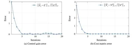
Fig.1 Robustness test of Procedure 3 whenΔG∞=0.2

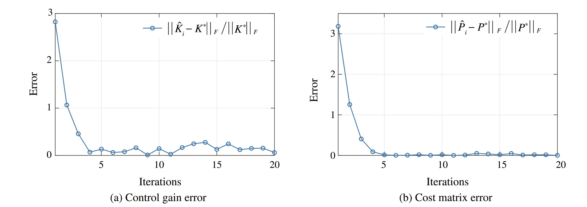
Fig.2 Robustness test of Procedure 4 whenΔM∞=0.2

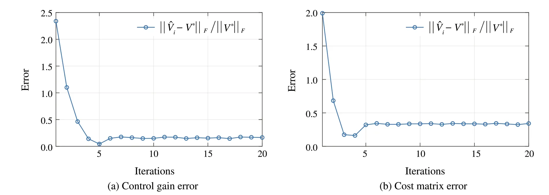
Fig.3 Robustness test of Procedure 6 when the noisy data is applied for the construction of ˆΛ

6 Conclusion

In this paper, we have studied the robustness property of policy optimization in the presence of disturbances at each iteration.Using ISS Lyapunov techniques,it is demonstrated that the PI ultimately converges to a small neighborhood of the optimal solution as long as the disturbance is sufficiently small.In this paper,we also provided a quantifiable bound.Based on the ISS property and Willems’fundamental lemma,a learning-based PI algorithm is proposed and the persist excitation of the exploratory signal can be easily guaranteed.A numerical simulation example is provided to illustrate the theoretical results.

Data availability The data that support the findings of this study are available from the corresponding author, L.Cui, upon reasonable request.