Distributed Nash equilibrium seeking with order-reduced dynamics based on consensus exact penalty

Shu Liang·Shuyu Liu·Yiguang Hong·Jie Chen

Abstract In this paper,we consider a networked game with coupled constraints and focus on variational Nash equilibrium seeking.For distributed algorithm design, we eliminate the coupled constraints by employing local Lagrangian functions and construct exact penalty terms to attain multipliers’optimal consensus,which yields a set of equilibrium conditions without any coupled constraint and consensus constraint.Moreover,these conditions are only based on strategy and multiplier variables,without auxiliary variables.Then,we present a distributed order-reduced dynamics that updates the strategy and multiplier variables with guaranteed convergence.Compared with many other distributed algorithms,our algorithm contains no auxiliary variable,and therefore,it can save computation and communication.

Keywords Game theory·Nash equilibrium seeking·Distributed algorithm·Coupled constraints·Order-reduced dynamics

1 Introduction

Distributed Nash equilibrium seeking for multi-player noncooperative games has been widely considered in many fields, such as robot swarm control [1], automatic driving[2],and charging scheduling[3].It aims to obtain an equilibrium strategy profile through players’own computation and communication,where each player uses only local data and neighbors’information over a network.Particularly,it is of interest for networked games,where the strategic interaction among players is consistent with the network[4].

Coupled constraints are widely considered in multi-agent systems,typically when the agents share limited resources.For example, [5] has considered coupled constraints in a distributed optimization problem and developed resource allocation algorithms.Moreover,players in a game can also have coupled constraints[6].It becomes a major problem to deal with coupled constraints in a distributed manner,since,for each agent or player, the others’ data and information associated with the coupled constraints are not fully available.

Generalized Nash equilibria are suitable for games with coupled constraints[7].Moreover,the variational Nash equilibrium is widely adopted as a refinement of the generalized Nash equilibria with many good properties [8].Recently, a few works have considered distributed variational Nash equilibrium seeking.For example,[9]has designed a distributed gradient-based projected algorithm and[10]has introduced a forward–backward operator splitting method.Also,[11]has considered distributed seeking dynamics for multi-integrator agents.

The game model with coupled constraints generalizes that of coupled constrained optimization,whereas some new difficulties occur.In the game model, multiple players are interacted and the corresponding equilibrium problem cannot be decomposed into independent optimization sub-problems.Consequently,some optimization theories and methods,such as the duality theory and penalty method, are not sufficient for games.In particular, it is well known that the Lagrangian function plays a key role for constrained optimization, which connects the primal and dual parts.In the game model, each player’s constrained optimization corresponds to a local Lagrangian function, whereas there is no commonLagrangianfunctionforallplayers.Hence,methods based on a single Lagrangian function,such as[12]for distributed coupled constrained optimization,cannot be directly used for the variational Nash equilibrium problem.

It is also of importance to simplify local dynamics in a distributed algorithm,since they are coordinated together with the complexity proportional to the network size.However,for problems with coupled constraints,distributed algorithm designrequirestoextend(oraugment)theproblemwithadditional variables to separate those couplings.For example,in addition to the strategy and multiplier variables, [9–11]have employed auxiliary ones in their distributed algorithms.An idea for simplifying distributed dynamics is to remove some updating variables so that the order of the dynamics can be reduced.In view of this, penalty methods are useful to transform a constrained problem into an unconstrained one to reduce the number of variables.In fact,[12]and[13]have used exact penalty methods to achieve order-reduced dynamics for distributed optimization problems,and[14]has adopted an inexact penalty method for the equilibrium seeking.

In this paper,we consider a networked game with coupled constraints and present a distributed variational Nash equilibrium seeking dynamics.Due to the coupled constraints,directly solving the variational Nash equilibrium requires global information.We mainly use two equivalent transformations to give equilibrium conditions that are suitable for distributed design and also achieve order reduction.Specifically,in the first transformation,we give a set of conditions in terms of local Lagrangian functions and eliminate the coupled constraints.In the second transformation,we construct exact penalty terms to render the optimal consensus of multipliers.In this way,we obtain equilibrium conditions without the coupled constraints and the consensus constraint.By simply using partial (sub)gradients, we construct a distributed dynamics to seek a solution to the transformed equilibrium problem, which contains the considered variational Nash equilibrium.Compared with existing works,a major feature of our method is that, instead of considering the first-order variational inequality problem that defines the variational Nash equilibrium, we focus on the zeroth-order objective functions of the multipliers,which makes it possible to use the exact penalty method to achieve order reduction.

The main contributions of our work are listed as follows.

1.Despite the absence of a common Lagrangian function for all players in the game,we obtain that the multipliers indeed correspond to a consensus optimization problem parameterized by the strategy variables.As a result,our method solves the variational Nash equilibrium seeking problem and extends the exact penalty-based method given in[12]for problems from coupled constrained optimization to coupled constrained game.

2.The equivalently transformed conditions we derive for distributed design contain only strategy and multiplier variables, whereas those in [9–11] also contained auxiliary variables.Accordingly, our distributed seeking dynamics is of lower order than those in[9–11].It updates no auxiliary variable and reduces the costs of computation and communication.

3.We construct exact penalty terms,which allow for constant and bounded penalty coefficients with guaranteed correctness.Accordingly, our seeking dynamics simply uses a constant coefficient.In comparison,the dynamics given in [14] based on an inexact penalty method must be equipped with time-varying and unbounded penalty coefficients.

The paper is organized as follows.Preliminaries are given in Sect.2, while the problem formulation is presented in Sect.3.Then,the main results about distributed design and analysis are given in Sect.4.Numerical results are presented in Sect.5,and the conclusions are given in Sect.6.

2 Preliminaries

In this section,we introduce relevant preliminary knowledge about convex analysis, variational inequality, differential inclusion,and graph theory.

2.1 Notations

Denote by Rnthen-dimensional real vector space and bythe nonnegative orthant.Denote by 0n∈Rnthe vectors with all components being zeros.For a vectora∈Rn,a≤0 means that each component ofais less than or equal to zero.Denote by ‖·‖ and |·| theℓ2-norm andℓ1-norm for vectors,respectively.Denote by col(x1,...,xN)the column vector stacked with column vectorsx1,...,xN, i.e.,col(x1,...,xN) =()T.Denote by sign(·) the sign function and by Sign(·)the set-valued version,i.e.,

2.2 Convex optimization and variational inequality

A setΩ⊆Rnis convex ifλz1+(1-λ)z2∈Ωfor anyz1,z2∈Ωandλ∈[0, 1].Denote by rint(Ω) the relative interior ofΩ.Denote bydΩ(·)andPΩ(·)the distance function and the projection map with respect toΩ,respectively.That is,

Denote byNΩ(x)the normal cone with respect toΩand a pointx∈Ω,i.e.,

A functionf:Ω→R is said to be convex iff(λz1+(1-λ)z2)≤λ f(z1)+(1-λ)f(z2)for anyz1,z2∈Ω,z1/=z2andλ∈[0, 1].

The following lemma presents a first-order optimal condition for constrained optimization,referring to[15,Theorem 8.15].

Lemma 1Consider an optimization with a convex objective function f and a convex constraint set Ω,i.e.,

Then,x∈Ω is an optimal solution if and only if

where ∂f is the subdifferential of f.

Moreover, we need the following result about exact penalty,referring to[16,Proposition 6.3].

Lemma 2Suppose that f has a Lipschitz constant κ0on an open set containing Ω.Then,the constrained optimizationminx∈Ω f(x)is equivalent to the unconstrainedminx f(x)+κdΩ(x)for any κ>κ0.Here,the equivalence means that they share the same optimal solution set.

Given a subsetΩ⊆Rnand a mapF:Ω→Rn, the variational inequality problem, denoted by VI(Ω,F), is to find a vectorx∈Ωsuch that

Its solution set is denoted by SOL(Ω,F).The mapFis said to be monotone overΩif

Moreover, it is strictly monotone if the inequality holds strictly wheneverx/=y.

The following lemma gives existence and uniqueness conditions for the solution to a variational inequality, referring to[17,Corollary 2.2.5 and Theorem 2.2.3].

Lemma 3If Ω is compact,thenSOL(Ω,F)is nonempty and compact.Moreover,if F is strictly monotone,thenSOL(Ω,F)is a singleton.

2.3 Graph theory

Graph of a network is denoted byG=(V,E),whereV={1,...,N}is a set of nodes andE⊆V×Vis a set of edges.Nodejis said to be aneighborof nodeiif(i,j) ∈E.The set of all the neighbors of nodeiis denoted byNi.The graphGis said to beundirectedif(i,j) ∈E⇔(j,i) ∈E.A path ofGis a sequence of distinct nodes where any pair of consecutive nodes in the sequence has an edge ofG.Nodejis said to beconnectedto nodeiif there is a path fromjtoi.Moreover,Gis said to be connected if any two nodes are connected.The detailed knowledge about graph theory can be found in[18].

3 Formulation

Consider a non-cooperative game over a peer-to-peer network with a graphG=(V,E),whereV={1,...,N}.For eachi∈V,theith player has a strategy variablexibelonging to a strategy setΩi⊂Rni,whereni> 0 is an integer.Also,the cost function of theith player isJi(xi,x-i),wherex-i= col(x1,...,xi-1,xi+1,...,xN) is the collection of other players’ decision variables.Here, we consider anetworked game, whereJi(xi,·) only depends on neighbors’strategy variablesx j,j∈Ni.

The strategy profilex= col(x1,...,xN) is within the direct product setΩ=Ω1×···×ΩN⊂Rn,wheren=n1+···+nN.Besides,there is a coupled constraint set

wheregi:Rni→Rp,i=1,...,Nwith an integerp>0.Theith player aims to minimize its cost function subject to local and coupled constraints,which can be written as

wheregi(xi,x-i)=g(x).

The variational Nash equilibrium of the considered game,referring to [7], is a solution to the variational inequality

VI(X,F),where

It is an acceptable solution for a game with coupled constraints.The relationship among the well-known Nash equilibria,generalized Nash equilibria,and the variational one is briefly explained as follows:

• If there is no coupled constraint,one can adopt aNash equilibriumpointxNE,at which no player can further decrease its cost function by changing its decision variable unilaterally in the local feasible set.That is, for eachi∈V,

• In the presence of the coupled constraint setC,theith player’s strategy should be within the setCi(x-i) ={xi∈Rni|gi(xi,x-i) ≤0p} that depends onx-i.Then, ageneralized Nash equilibriumpointxGNEattains the coupled constrained optimality

• Furthermore,there may be multiple generalized Nash equilibria,and among them,the variational Nash equilibrium pointxVE∈SOL(X,F) is widely used as a refinement[8].One advantage of the variational Nash equilibrium compared with other generalized Nash equilibria is that small feasible perturbations(not necessarily unilateral perturbations) aroundxVEdo not decrease any one of the cost functions[7].

Our goal is to compute a variational Nash equilibrium in a distributed manner.That is, for eachi∈V, theith agent updatesxiby using only local data and neighbors’information over the network.

To guarantee the existence of a solution to VI(X,F)and the correctness of distributed algorithms,a few basic assumptions are adopted as follows;

A1:Ωis compact and convex,gi,i=1,...,Nare convex and differentiable,andFis strictly monotone.

A2: 0 ∈rint(Ω-C).

A3: The network graphGis connected.

Here,A1 guarantees the existence and uniqueness of the variational Nash equilibrium according to Lemma 3, and A2 resembles the Slater’s constraint qualification.Note that the monotonicity ofFimplies the convexity ofJi(·,x-i) for eachi∈V.In addition, A3 is widely used for distributed algorithms in the literature.

Remark 1Regardingthecoupledconstraints,[9]and[10]has considered affine equality and inequality ones,respectively.Here,we consider nonlinear and inequality ones as same as thosein[11],whichistechnicallyharderthantheaffinecases.Also,regardingthemonotonicity,[9–11]haveadoptedstrong monotonicity, while we adopt a less restrictive assumption with only strict monotonicity.

Remark 2The considered coupled constrained game is more general than coupled constrained optimization.In fact,whenJi(xi,x-i) =f(x) =f1(x1)+···+fN(xN), ∀i∈V, it is not difficult to verify that the variational Nash equilibrium problem reduces to the optimization problem

as considered in[5,12,19,20].

4 Main results

In this section,we present our distributed design and analyze the proposed algorithm.

4.1 Algorithm design

Our design is given in Algorithm 1.

In Algorithm 1, theith player updates its variables by using local and neighbors’ information.Thus, it is a distributed algorithm.Our dynamics involves discontinuous right-hand side caused by a few sign functions,and its solution is understood in the sense of Filippov,referring to[21].To be specific, forλ= col(λ1,...,λN), the discontinuous map

is regularized to a set-valued map

whereμ(·)is the Lebesgue measure andB(λ,δ)is the ball centered atλwith radiusδ.We need explicitly characterizeF[γ], since it is utilized to analyze the trajectory solution.Note thatF[γ]is not equal to

In fact,

By the generalized gradient formula[16,Theorem 8.1],it is not difficult to obtain that

where

Therefore,the compact and regularized form of (4)is

which will be used in our analysis.

Remark 3Dynamics(3)and(4)are of orderniandp,which are associated with theith player’s strategy and multiplier.In comparisons,many other distributed algorithms,such as the continuous-time ones [1, 11, 22] and the discrete-time ones [10, 23], involve additional dynamics of orderpwith respect to auxiliary variables.For example,the discrete-time algorithm given in[10]is written as

Also,the continuous-time algorithm given in[11]is written as

Clearly, Algorithm 1 reduces the order of theith player’s dynamics fromni+2ptoni+p.

Remark 4The distributed algorithm given in[14]is written as

whereP(·)is an inexact penalty term to deal with inequality constraints, andς(t),δ(t),ε(t),γ(t) andw(t) are timevarying parameters of the form(1+t)a.These parameters are time-varying and unbounded.Also,the order of this dynamics isn1+···+nN,since it estimatesx-iusing variablesyi j,j∈V{i} to calculate the values of the coupled constraint functions.In comparison,our dynamics uses simply a constant parameterαand does not introduce additional variables to estimatex-ifor the coupled constraints.

4.2 Equilibrium conditions

Different from focusing on the variational inequality problem with (2), we alternatively characterize the variational Nash equilibrium using local Lagrangian functions associated with(1).These functions have also been discussed in[7].

Lemma 4Under A1–A3,a point x∈Ω is the variational Nash equilibrium if and only if there exists a multiplier λ∈such that

where

ProofThe equivalence between VI(X,F)andL-based optimization characterizations follows from the fact that they share the same KKT conditions:

This completes the proof.■

Lemma 4 removes the coupled constraint setCby using a set of equilibrium conditions in terms ofLi,i=1,...,N+1.However,they cannot lead to distributed design,since they use the coupled constraint functionsg(x) and a common multiplierλ.Therefore, we use an exact penalty technique to modify these Lagrangian functions with local multipliers and decompose the constraint functions as follows.

Theorem 1Under A1–A3,a point x∈Ω is the variationalNash equilibrium if and only if there exists λ∈such that

where

with φ(·)in(5)and α satisfying

ProofBy Lemma 4,we need only to prove that(x,λ)satisfies(7)if and only if

The“if”part can be easily verified,and we focus on the“only if”part.By(7),λsolves

We claim that it shares the same optimal solutions with

where

Comparing(8)with(9),αφ(λ)acts as a penalty term associated with the constraint setΛ.Moreover,if this penalty is exact,then the equivalence between(8)and(9)holds.Since the objective function in (9) isκ0-Lipschitz continuous, it follows from Lemma 2 thatKdΛ(λ)is an exact penalty term for anyK>κ0.Thus,to verify thatαφ(λ)is also an exact penalty term,it suffices to prove

By calculations,

Since the graph is connected and undirected,there is a path connecting nodeskandlfor anyk,l∈V.As a result,

Consequently,

which implies

This completes the proof.■

Remark 5Theorem1indicatesthatthepenalty-basedmethod guarantees the consensus of multipliers.Removing this consensus constraint leads to a dimension-reduced problem,which establishes the foundation to design order-reduced seeking algorithms.Theorem 1 extends the penalty method associated with multipliers for distributed coupled constrained optimization given in [12].Here, we further deal with the game with coupled constraints and prove the equivalence between the two sets of equilibrium conditions(6)and(7),though no common Lagrangian function is available to establish a whole primal or dual optimization problem.

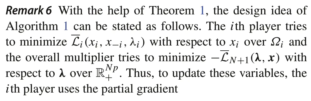
while the overall multiplier uses the partial subgradient

Here,the overall multiplier’s update requires no central node in the network.It is component-wisely updated by the associated players to make the algorithm distributed.

4.3 Convergence analysis

Algorithm 1 can be written in a compact form as

whereθ=col(x,λ),θ=col(x,λ)and

The correctness of its equilibria is presented as follows.

Theorem 2Under A1–A3,if θ and θsatisfy

then x is the variational Nash equilibrium.

ProofSince

there holds

That is,

and

According to Lemma 1,these are first-order optimal conditions for the minimizations in (7),which indicates thatxis the variational Nash equilibrium.■

With the correctness of the algorithm’s equilibria,we further verify the convergence of Algorithm 1.

Theorem 3Under A1–A3,the trajectories xi(t),λi(t),xi(t),λi(t)of Algorithm 1 are bounded for each i∈V.Moreover,x(t)converges to the variational Nash equilibrium.

ProofAn algorithm in the same form as(10)has been analyzed in our previous work[24](for another game problem),where the boundedness can be guaranteed if the mapΦis monotone.Moreover,the convergence can be guaranteed if the mapF(i.e.,partial gradients of players’cost functions)is strictly monotone.Thus,we need only to prove the monotonicity ofΦand omit repetition parts.

The mapΦcan be decomposed as

where

Sinceφis convex, its subdifferential is monotone.Thus, it suffices to prove the monotonicity ofΦoverΘ.To this end,for anyθ,θ′∈Θ,we analyze

where

Rearranging the terms with respect toλiandλ′iyields

By the monotonicity ofF,

Also,by the convexity ofgiand the positiveness ofλi,λ′i,

which impliesG(θ,θ′)≥0.Therefore,

As a result, the overall mapΦis monotone overΘ.This completes the proof.■

Remark 7Theorems 2 and 3 prove that Algorithm 1 solves the considered variational Nash equilibrium seeking problem.To be specific, Theorem 3 ensures that the trajectoryθ(t)of(10)converges to an equilibrium pointθ∗=(x∗,λ∗),and Theorem 2 ensures the correctness of this point in thatx∗is the variational Nash equilibrium.

5 Numerical examples

In this section, we give numerical examples for illustrating our obtained results.

Example 1To show the effectiveness of our algorithm, we compare its performance with some others.Consider a non-cooperativenetworkedgamewith4playersandthecommunication graph is shown in Fig.1.The objective functions are

Fig.1 The communication graph of four agents

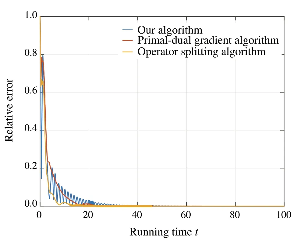
Fig.2 The comparison of relative errors

To seek the variational Nash equilibrium of this game,our algorithm, the primal-dual gradient algorithm given in[11], and the operator splitting algorithm given in [10] are utilized(see also Remark 3 for the latter two algorithms).The trajectories of relative error are shown in Fig.2.The orders of these three algorithms are summarized in Table 1.Clearly,all these algorithms can solve the variational Nash equilibrium,and our algorithm has lower order than the others.

Inaddition,wealsotrytomakecomparisonswiththealgorithm given in[14](see Remark 4).However,this algorithm uses time-varying penalty parameters in the form of(1+t)a,and the corresponding discrete-time approximation using the forward Euler difference method with the same stepsize as ours is divergent.Also,if the time-varying penalty parameters are replaced by bounded constants,our simulation shows that the obtained solution does not satisfy the constraints.

Example 2Consider the power control problem of a multiuser cognitive radio system, referring to [25].A multi-usercognitive radio system consists ofNcognitive users who share licensed resource over frequency-selective channels withnsubcarriers.Theith user assigns powerx(ℓ)ito the channel with subcarrierℓto enable its communication in the presence of noise and interference from other users.The rate of theith user is

Table 1 The comparison of the order of algorithms

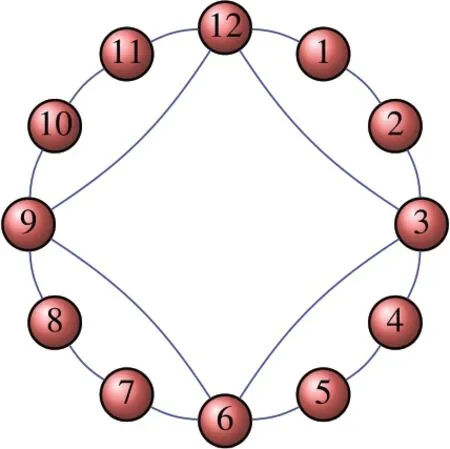
Fig.3 The communication graph of twelve agents

The constantsare magnitudes of channel transfer functions, and the constantsare the powers of noises.Moreover,a prerequisite of the spectrum sharing is that the users can only introduce limited total interference to the system,which leads to the set of coupled constraints as

•N=12 andn=4.

•Ωi=[0,1]n, ∀i∈V.

•Isum=0.25Nn,andIind(ℓ)=0.5N,∀ℓ=1,...,n.

• The network graph is shown in Fig.3.

• The datav(ℓ)iare randomly generated from[0.5,1.5].

The simulation results are shown in Figs.4–6.In particular,Fig.4 shows the convergence of the profilex(t)and Fig.5 shows the convergence and consensus ofλ(t).Also, Fig.6 shows thatg(x(t))becomes less or equal to the zero vector eventually,which renders the coupled constraintsg(x)≤0p.

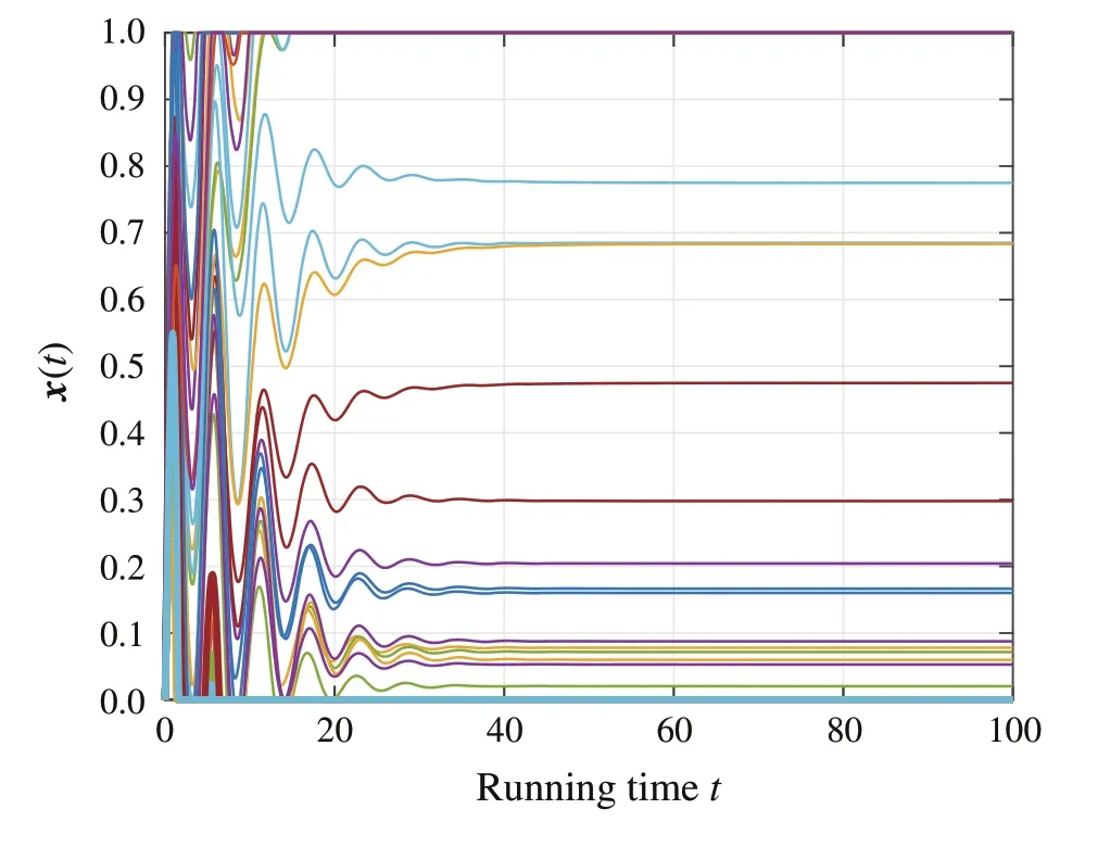
Fig.4 The trajectories of the profile x(t)

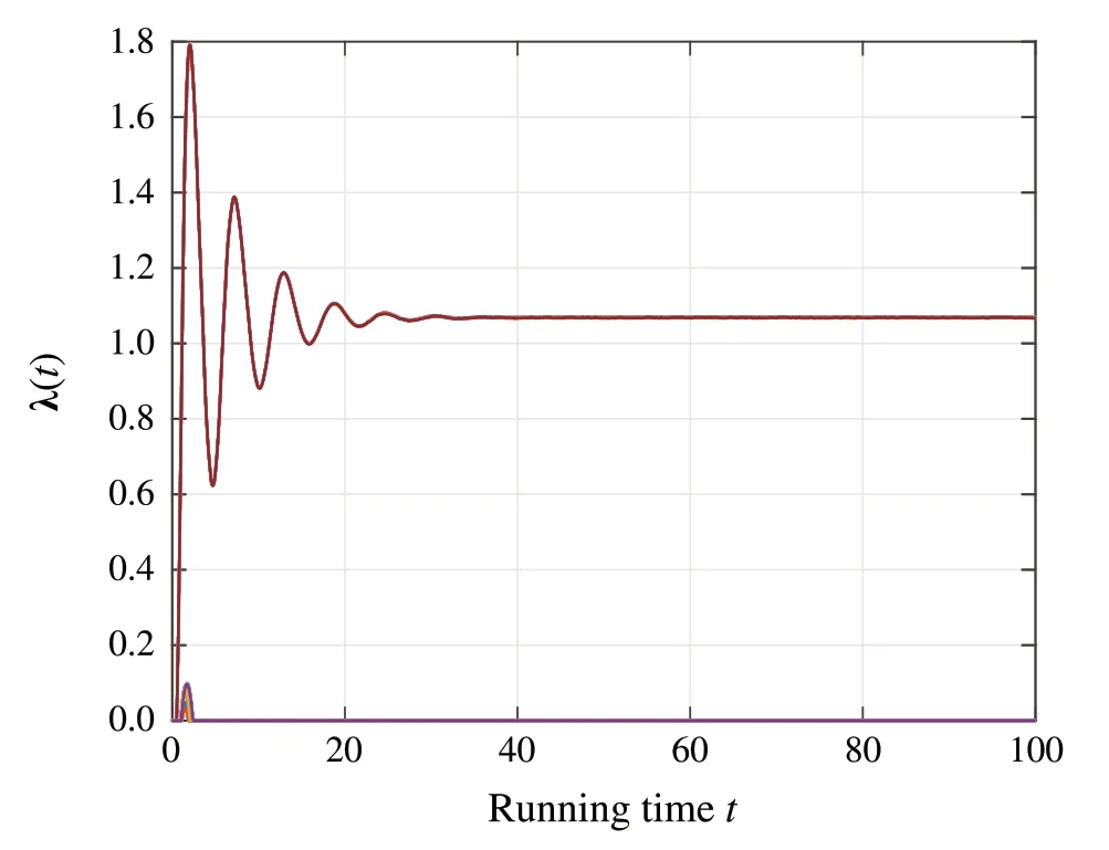
Fig.5 The trajectories of the multiplier λ(t)

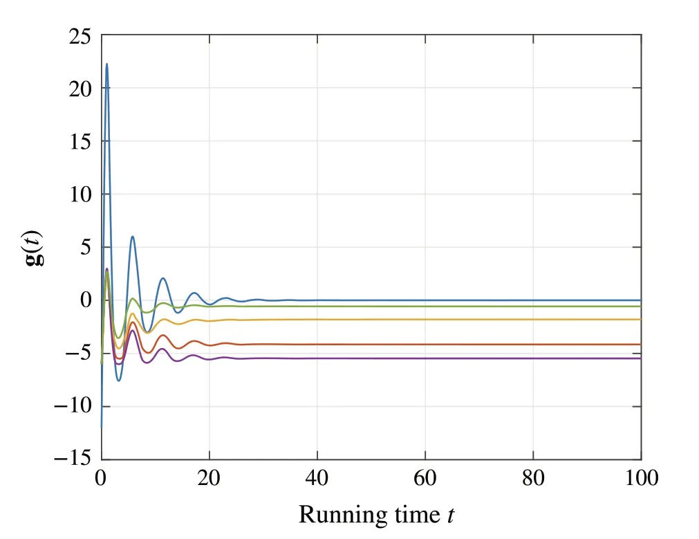
Fig.6 Values of the constraint functions g(t)= g(x(t))

6 Conclusions

In this paper,a distributed variational Nash equilibrium seeking algorithm has been proposed for a networked game with coupled constraints.An order-reduced dynamics has been designed to update strategy and multiplier variables with guaranteed convergence.In comparison with some existing distributed ones, our algorithm has saved the computation and communication.This reduction has been achieved using an exact penalty method to guarantee the consensus of multipliers, even though no common Lagrangian function is available.Future works may include a further application of our developed technique to complicated distributed design.