Adaptive data fusion framework for modeling of non-uniform aerodynamic data

Vinh PHAM, Mxim TYAN,, Tun Anh NGUYEN, Chi-Ho LEE,L.V.Thng NGUYEN, Je-Woo LEE,,

a Department of Aerospace Information Engineering, Konkuk University, Seoul 05029, Republic of Korea

b Konkuk Aerospace Design-Airworthiness Institute, Konkuk University, Seoul 05029, Republic of Korea

KEYWORDS Aerodynamic modeling;Data fusion;Diverse data structure;Multi-fidelity data;Multi-fidelity surrogate modeling

Abstract Multi-fidelity Data Fusion (MDF) frameworks have emerged as a prominent approach to producing economical but accurate surrogate models for aerodynamic data modeling by integrating data with different fidelity levels.However, most existing MDF frameworks assume a uniform data structure between sampling data sources;thus,producing an accurate solution at the required level,for cases of non-uniform data structures is challenging.To address this challenge,an Adaptive Multi-fidelity Data Fusion (AMDF) framework is proposed to produce a composite surrogate model which can efficiently model multi-fidelity data featuring non-uniform structures.Firstly,the design space of the input data with non-uniform data structures is decomposed into subdomains containing simplified structures.Secondly, different MDF frameworks and a rule-based selection process are adopted to construct multiple local models for the subdomain data.On the other hand,the Enhanced Local Fidelity Modeling(ELFM)method is proposed to combine the generated local models into a unique and continuous global model.Finally,the resulting model inherits the features of local models and approximates a complete database for the whole design space.The validation of the proposed framework is performed to demonstrate its approximation capabilities in (A) four multi-dimensional analytical problems and (B) a practical engineering case study of constructing an F16C fighter aircraft’s aerodynamic database.Accuracy comparisons of the generated models using the proposed AMDF framework and conventional MDF approaches using a single global modeling algorithm are performed to reveal the adaptability of the proposed approach for fusing multi-fidelity data featuring non-uniform structures.Indeed,the results indicated that the proposed framework outperforms the state-of-the-art MDF approach in the cases of non-uniform data.

1.Introduction

Data fusion produces an integrated database from multifidelity data sources to obtain more consistent, accurate, and synthetic information than any individual1.In data fusion,surrogate models have been used to produce economic approximation models based on available samples to accurately predict specific data under consideration at an acceptable cost.In aerospace engineering, data fusion techniques are often adopted to construct an Aerodynamic Database (AeroDB)for aircraft design optimization and flight simulation.An AeroDB is strictly required to be precise and extensive to provide the aerodynamic coefficients of vehicles for various flight conditions and vehicle configurations throughout the whole mission.Nevertheless, the AeroDB is constructed using a set of analysis tools with different fidelity levels under different computational schemes because each tool is usually only valid for a specific analytical condition2.Generating an extensively large-sized database based on high-fidelity methods, such as flight testing, wind tunnel testing, or Ansys Fluent RANS CFD (CFD) simulation, is challenging due to costly and time-consuming computation.That may make a direct construction of an AeroDB impossible due to budget and time limits.Furthermore,using a simplified model of the actual system may reduce the accuracy of the resulting data.

Therefore, surrogate-based data fusion is an economical and efficient approach to constructing aerodynamic models for mining data to resolve the abovementioned challenges.Renowned single fidelity surrogate modeling methods include polynomial Response Surface Modeling (RSM)3–5, Radial Basis Function neural networks (RBF)6,7, kriging8–10, and Artificial Neural Network (ANN)11–13, and they are often used to construct an approximation model from a single sampling set.However, the quality of surrogate models is considerably influenced by the number of training sample points.The surrogate models need a certain number of training samples to achieve a converged accuracy.Indeed, fewer sample points may reduce the computational cost but lead to an inaccurate model.

To significantly reduce the required number of HF sampling data, a large number of Multi-fidelity Data Fusion (MDF)frameworks have been developed to fuse a set of Low-Fidelity(LF) sampling data along with a small amount of High-Fidelity (HF) sampling data, to obtain a more accurate database compared to either the original LF or HF data.Here,the LF data can be exploited in significant quantities from simplified models or low-cost analyses.Specifically, a variety of MDF frameworks, such as co-kriging14–16, Global Variable-Fidelity Modeling (GVFM)17–21, Hierarchical Kriging (HK)22,23, Improved Hierarchical Kriging (IHK)24, or co-ANN 25,26adopt two multi-fidelity datasets to construct an approximation model and generate a multidimensional database.Extended Co-Kriging (ECK)27,28and Linear Regression Multi-Fidelity Surrogate Modeling (LR-MFSM)29simultaneously use a multitude of non-hierarchical LF datasets to provide more information during the construction of an HF model.

However, the nature of the existing MDF frameworks in previous studies assumes that the structure of sampling datasets is uniform or that the distribution domains of sampling plans are globally coincident in a design space.Furthermore,these methods are mostly used for interpolation.Nevertheless,when the distributions of sampling plans are non-uniform,which causes the existence of different data structures in each local domain of the design space.The number of data sources in each local domain may be different.It is often challenging to construct an accurate model for the whole design space solely using the methods mentioned above due to the inevitable involvement of extrapolation in voids or the local regions’missing HF data.From a practical standpoint,the data fusion problems for database generation raises the following two challenges30:

(1) Multidimensional interpolation/extrapolation: capability to cover a database for the whole design space based on scattered and discretized input data.

(2) Multiple data mixtures: capability to develop a consistent and homogeneous aerodynamic database from multi-fidelity data with non-uniform structures.

To resolve the above challenges,an Adaptive Multi-fidelity Data Fusion (AMDF) framework is proposed to efficiently construct a global surrogate model using a multitude of multi-fidelity datasets, notably featuring non-uniform data structures.The global model is developed by simultaneously integrating multiple local surrogate models.Moreover, the interpolation and extrapolation are handled by optimal solutions.Furthermore, the design space of the input datasets is subdivided into subdomains with more superficial structures.This technique uses traditional surrogate modeling methods to build several local models for each subdomain.We propose an Enhanced Local Fidelity Modeling (ELFM) method to construct a unique global model by combining the generated local models.This global model retains the attributes of the local models and approximates a complete database for the entire design space.Finally, the approximation performance of the proposed method is illustrated through four analytical examples and a practical aerospace application example.A more accurate global surrogate model can be obtained from the AMDF framework than the four conventional methods.

A comprehensive analogy of different related works in the literature, previously mentioning specific aspects, including(A) the data structure, (B) the number of fidelity levels (LF,HF),(C)the number of outputs,and(D)the inter/extrapolation adoptability, is shown in Table 13,6,7,9,10,14–16,19,20,22,24,26–41.In AeroDB database construction, the ultimate objective is to develop a global model that involves all available datasets.However,the possibility of different data structures,especially non-uniform data, is commonly high in engineering.Moreover, the final goal of the AeroDB generation is to obtain a surrogate model with high adoptability for interpolation and extrapolation on multi-dimensional data featuring diverse data structures.

Most MDF frameworks have been developed for data fusion problems with uniform data structures.There are still a relatively small number of efficient MDF frameworks for non-uniform data.Recently, Belyaev et al.30developed an MDF framework known as the Local Fidelity Modeling(LFM) for a specific spacecraft aerodynamic database construction, comprising diverse fidelities of non-uniform data.The study proposed weight functions as bridge functions to integrate two separate surrogate models into a single global model and transfer local information from the component models to the global model based on the distribution of sample points.However, in the case of uniform data, the approach does not always result in a reasonable approximation model from a physical standpoint.In one of the most recent studies,Liu et al.31proposed the Multi-Fidelity Gaussian Process(MFGP), a Bayesian discrepancy MDF framework.TheMFGP is composed of a global trend term and several local residual terms,enabling the transfer of shared global and local features from the LF model to the HF model.The approach,meanwhile, requires a significant amount of effort to estimate several model parameters.Lin et al.32proposed a Multi-fidelity Multi-output Gaussian Process (MMGP) model as a global model exploiting both the information of LF models and the transferred information across several HF outputs to construct an HF model.On a different approach,instead of using a global algorithm to construct a global model for the entire design space directly, the proposed method implements a multi-stage process to divide the design space into subdomains and construct separate local models with optimal modeling methods.The global model is then constructed by flexibly and comprehensively integrating local models into a unique smooth model.

Table 1 Analogy of MDF frameworks.

Upon the above analogy, this work extends the related research area on data fusion methodologies through the following key contributions:

(1) We proposed a novel AMDF framework as an automated process to efficiently solve diverse data fusion problems in modeling multi-fidelity and non-uniform data.The framework features a rule-based selection process of different surrogate models and MDF frameworks, thus enabling designers to model design problems efficiently and objectively without a deep knowledge of the input data structures.

(2) We proposed an ELFM method as the backbone of the model construction in the AMDF framework, allowing the fast integration of multiple discretized local models into a unique and smooth global model.

(3) We proposed optimal solutions in data fusion problems,particularly in the subdomains which require interpolation or extrapolation.The framework adaptively adopts a specific optimal surrogate modeling method to obtain the highest accuracy of the corresponding local model.The adaptive approach significantly improves the quality of the final global model and its generated database compared to conventional approaches, which fix a unique surrogate modeling method throughout the global model construction process of all data in the entire design space.

(4) We adopted the proposed framework of database construction in different data fusion problems, including(A) four multi-dimensional analytical problems and(B) an F16C fighter aircraft’s aerodynamic database generation for developing its digital twin.The results highlight the betterment of the proposed framework in producing a more accurate database compared to conventional approaches.

The outline of this manuscript is as follows:Section 2 introduces the format of data fusion problems and challenges.The details of the proposed framework are discussed in Section 3.For verifying the study, four analytical examples and an engineering case study are provided to validate the proposed method in Section 4.The advantages and disadvantages of the study and future works are discussed in Section 5, and the last section concludes the paper.

2.Background and terminology

Approximation problems require constructing a cheap-toevaluate surrogate model ^f(x ）that emulates the expensive response of a black box f (x ）.10,15Here f(x ）:Rm→R is a continuous quality, cost, or performance metric of a product or

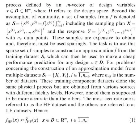
The sampling plans of these training datasets may be distributed in different domains in the design space,causing existing non-uniform data structures to occur in the design space.Voids and overlapping structures probably exist between the distribution domains of the sampling plans.Fig.1 demonstrates a general data fusion process to construct a database from multi-fidelity data.At the end of the process, the resulting model can approximate the HF samples and perform interpolation and extrapolation for any untried points to construct a homogeneous and accurate database.

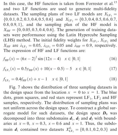
One of the peculiarities of a data fusion problem considered in this work is an input of multi-fidelity data featuring nonuniform structures.Fig.3 shows an example of a training dataset, which is a union of two sampling plans distributed in different domains of the design space.

Such designs are complicated for surrogate modeling methods, which lack prior knowledge about the data structure.Indeed, conventional MDF methods assume that the structures of sampling plans are relatively uniform and that there are no voids in the design space to avoid oscillation and extrapolation.Hence, the AMDF framework is proposed to handle such a problem in the following section.

3.Proposed AMDF framework

The AMDF framework is proposed to efficiently produce a global surrogate model from multi-fidelity data with diverse data structures.The concept of the proposed approach assumes that (A) in any local domains of the design space,the data source with the highest fidelity is considered as the HF data in its local domain and the global model will follow its features; (B) extrapolation should only be performed in voids.The overall framework of AMDF is presented in Fig.4.Specifically,engineering data fusion problems start with the input of multi-fidelity training datasets.The detailed information about sampling points, the size of sampling plans, the number of dimensions, the boundaries of distribution domains,and the levels of fidelity are all specified(Section 3.1).Then, the features of the training data datasets are analyzed(‘Data Analysis’- Section 3.2) to recognize the scenarios of the data structures based on the parameters: (A) the number of fidelity levels and (B) the distribution domains of datasets in the design space.

Fig.1 General setup of a data fusion problem for a database construction.

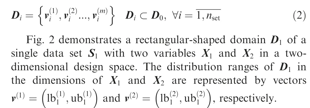
Fig.2 Distribution domain and boundaries of a sampling plan in a two-dimensional design space.

Fig.3 Sampling plan with multiple sources and non-uniform distribution.

This article proposes four typical scenarios to describe all possible data structures in data fusion problems.Two scenarios(Types I and II)demonstrate uniform data structures,while the other ones (Types III and IV) demonstrate non-uniform data structures.Details of the typical scenarios are described in Section 3.2.1.It is assumed that the input datasets have one of the scenarios of uniform data structures, then they are sent directly to the ‘Multi-fidelity surrogate model construction’(Section 3.3) to produce a global model with the optimal selection from the available surrogate model methods,according to each corresponding scenario.In contrast,the scenarios with non-uniform data structures would be sent to the ‘Domain decomposition’(Section 3.2.2).Then, the initial training datasets are decomposed into multiple subsets with uniform structures according to different local regions or subdomains.After that, subsets of each subdomain are sent back to the starting point of the framework to begin new processes of constructing local models for each subdomain.Then, constructed local models are assembled into a unique global model using a special technique called the Enhanced Local Fidelity Modeling (ELFM) method (Section 3.3.2).The resulting global model can be used to confidently interpolate untried data located in the distribution domains of training datasets.However,if large voids exist or the distribution domains of training datasets do not cover the entire design space, it requires extrapolation to construct a complete database.In this case,the global model needs an additional process to enhance its extrapolation performance in the‘Extrapolation enhancement’(Section 3.3.3).The final global model can confidently interpolate/extrapolate an accurate database for any untried points in the design space.

3.1.Input data

The features of a particular data fusion problem are reflected in its input data features.Besides the sample points,the following features of the training datasets should be investigated.

(1) Size of input data: The size of the input data for a particular problem denotes the number of datasets from different sources contained in the input dataset.

(2) Dimensionality: The number of dimensions denotes the input variable dimension or the number of variables.

(3) Distribution domain:The distribution domain of a dataset is determined by the boundaries of the corresponding sampling plan in the design space.Hence, different distribution domains exist in the design space for the input of multi-fidelity data.

(4) Level of fidelity: The input sampling data may contain multiple sampling datasets with different levels of fidelity.However, the distinction of fidelity levels is based on the user’s comprehensive knowledge and assumption of the nature of data sources.To quantify this assumption on the fidelity levels of the datasets,the fidelity factor, λ, is introduced to represent the user’s confidence about the accuracy of the source that produces the response values at given points.The more important the information of the dataset is, the higher the fidelity weight value gains.For input data containing multiple data sets with different fidelity levels:

where λiis the fidelity weight of each dataset.Commonly,fidelity weight of a HF dataset should be initially set with a value of 0.9.The fidelity weights of lower-fidelity datasets can be set according to the condition given in Eq.(3).

3.2.Data analysis

3.2.1.Scenario recognition

This work proposes four typical data fusion scenarios to describe possible input data structure scenarios.Each scenario is distinguished according to two criteria: the number of fidelity levels (single or multiple) and the correlation between the domains of the sampling plans(separate,overlapping,or coincident).Hence, Fig.5 demonstrates simple examples of four typical scenarios, in the case of two-dimensional data with variables X1and X2.It is assumed that there are two different sampling datasets S1and S2with different fidelity levels and corresponding distribution domains of sampling plans D1and D2, respectively.The boundaries of distribution domains are illustrated by rectangles.Fig.5(a) shows a demonstration of a Type I scenario.The input data contains a single data set with the distribution domain D1.The problem requires the construction of a database by interpolating new data at untried points in the domain D1.A Type II scenario, shown in Fig.5(b), has two different datasets with different fidelity levels, including the LF dataset, S1and the HF dataset, S2,with the corresponding domains D1and D2.All domains are coincident (D1≡D2).It requires interpolating the new HF data at untried points inside the available domain.The scenario can be extended to adopt an HF dataset and multiple LF datasets.Fig.5(c)demonstrates a Type III scenario,which has multi-fidelity input data.Unlike the Type II scenario,distribution domains D1and D2are separated (D1∩D2=ø).The information of each dataset is independent and has the highest fidelity in its local distribution domain.The problem requires evaluating untried points between two domains and the void zone.Fig.5(d) demonstrates a Type IV scenario.The input contains two data sets with overlapping distribution domains.The problem requires both interpolation and extrapolation at untried points in the whole design space.Type I and Type II are considered fundamental interpolation problems, while the Type III and Type IV are complex problems accounting for both interpolation and extrapolation works.

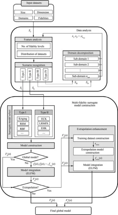
Fig.4 AMDF framework process.

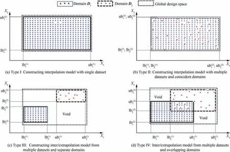
Fig.5 Typical scenarios of data fusion problems featuring prediction requirement, number of input datasets and correlation between distribution domains.

Indeed, the typical problems can be recognized from the input problem without directly observing all data points.The Type I problems can be easily recognized by checking if the number of datasets contained in the input data is single or multiple.With multi-fidelity data scenarios(Type II,Type III,and Type IV), the recognition is performed by checking the existence of any overlapping between distribution domains.The distribution domains of the datasets are considered to overlap if there exists at least a lower or upper bound of a dataset domain in the distribution domains of the other datasets in every dimension.The condition can be expressed as follows:

The domains are separated if the condition in Eq.(4)is not satisfied.Thus,the structure of the input datasets fits the Type III scenario.Otherwise, it can be a Type II or Type IV scenario.The recognition is continued by checking if domains are coincident or partly overlapped.The condition to check coincident domains is that all boundaries of the domains are coincident in every dimension or:

If the condition in Eq.(5) is satisfied, the data structure of the input problem is characterized by a Type II scenario.Otherwise,the data domains overlap is characterized as a Type IV scenario.

3.2.2.Domain decomposition

For input datasets with data structures featuring Type III and Type IV scenarios,the design space is decomposed into different subdomains so that the data in each subdomain has uniform structures featuring Type I and Type II scenarios.Hence, the initial problem of constructing a surrogate model for the whole design space is converted into multiple subproblems to construct various local models for each subdomain of the design space.The domain decomposition is implemented using Algorithm 1.

Algorithm 1 (Obtain coordinates of decomposed subdomain).

A demonstration of domain decomposition is given in Fig.6; the process is applied to the example introduced in Fig.5(d).The input data contains two datasets S1and S2with different levels of fidelity.The domains D1and D2overlap each other.The determination of subdomains, decomposed from given primary domains,is shown in Fig.6(a).As a result,subdomains d1,1,d1,2,d1,3,d2,1,d2,2,d2,3,d3,1,d3,2,d3,3are decomposed from initial domains D1and D2.It is observed that subdomains d1,1,d1,2,d2,1contain samples only belonging to S1, while d2,3,d3,2,d3,3contains samples only belonging to S2.Subdomain d2,2simultaneously contains samples belonging to both data sets S1and S2It should be noted that subdomains d1,3and d3,1are empty subdomains;however,the data in these domains can be extrapolated using an extrapolation model constructed in the final stage of the AMDF process.Each subset is sequentially re-input to the AMDF process to construct local models.Thus, the number of local models to be constructed equals the number of subdomains, causing high computational costs.However, these obstacles can be minimized by merging adjacent subdomains containing the same data structures into a single domain to reduce the number of subdo-

3.3.Multi-fidelity surrogate model construction

3.3.1.Surrogate model selection

The surrogate model selection problem requires determining the best choice of surrogate model algorithms for the available data according to the scenario of data structures.This work uses a rule-based selection process developed by Jia et al.42to construct and evaluate various possible options of surrogate model algorithms for a particular scenario of input datasets.The most accurate model will be output as the final surrogate model for the input problem or the corresponding domain of the input datasets.The accuracy metric used for the evaluation is cross-validation root mean square error RMSELOOCV, the smaller RMSELOOCVthe more accurate the model.The expression of RMSELOOCVis:

where yiis the response of sample point xi, ^f( xi）denotes the predicted response for xiusing the model based on the current sample set, with the sample point xiremoved, and nxdenotes the total number of samples.

This paper focuses on adopting single-output modeling methods to reduce the computational complexity of numerical experiments to construct the global model.With each typical scenario of data fusion, there are multiple options for model selection.For a specific problem, the variants of RSM, RBF,and Kriging models are used to construct an approximation model for problems in a Type I scenario.The variants of RSM model types are different options for model orders.With the RBF model type, there are various options for the basic functions.In the Type II scenario,the two choices of surrogate model selection are ECK27and LRMFS29.The ECK is an extended version of co-Kriging, and both ECK and LRFMS can adopt the data from high-fidelity and multiple lowfidelity models.The detailed surrogate models in the selection pool are described in Table 2.

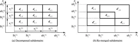
Fig.6 Domain decomposition process for example in Fig.5(d).

3.3.2.Model integration

In this work, the Enhanced Local Fidelity Modeling (ELFM)method is proposed, allowing the integration of multiple local models into a unique global model with a smooth connection.The method is inspired by the original LFM method proposed by Belyaev et al.30.It is assumed that the sampling data sets in the different subdomains diare approximated by local models fi.The global model︿Fgis the weighted sum of the local models

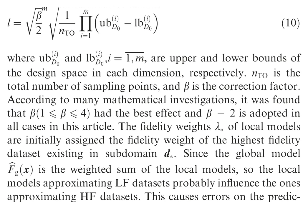
where wiare the weight functions of the local models,presenting their influence on the predictive point x,nsubis the number of local models, ψ(x ）*is the correlation model, X-*is DoE in each the subdomain digenerated using the Full Factorial Design of experiment (FFD) method.X-*represents the influenced domains of the corresponding local models on the global model.The scaling factor l is estimated as:

3.3.3.Extrapolation enhancement

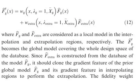
The global model ︿Fgneeds an efficient enhancement to extrapolate unknown data in void zones.To do that, an additional model ︿Fextrais constructed using extrapolation methods.Then,the resulting model ︿Fextrais integrated with the model ︿Fgto produce a final global model ︿Feg, which can be used for both interpolation and extrapolation.Previous works reported that,compared to kriging and RSM models43–45, neural networkbased models can have outstanding performance in extrapolation.Xu et al.33indicated that a neural network can extrapolate well when the activation function has a similar shape as the target function.In this work, extrapolation model ︿Fextrais constructed using an RBF neural network.Indeed, the RBF neural network has attracted much attention in various fields due to its simple structure, strong nonlinear approximation and good generalization46.Activation functions in RBF networks are radial basic functions.This work proposes using multi-quadric, linear, cubic, and thin-plate functions in the selection pool, to handle cases of linear or non-linear target functions.The detailed algorithm of model enhancement for extrapolation is described in Algorithm 2.

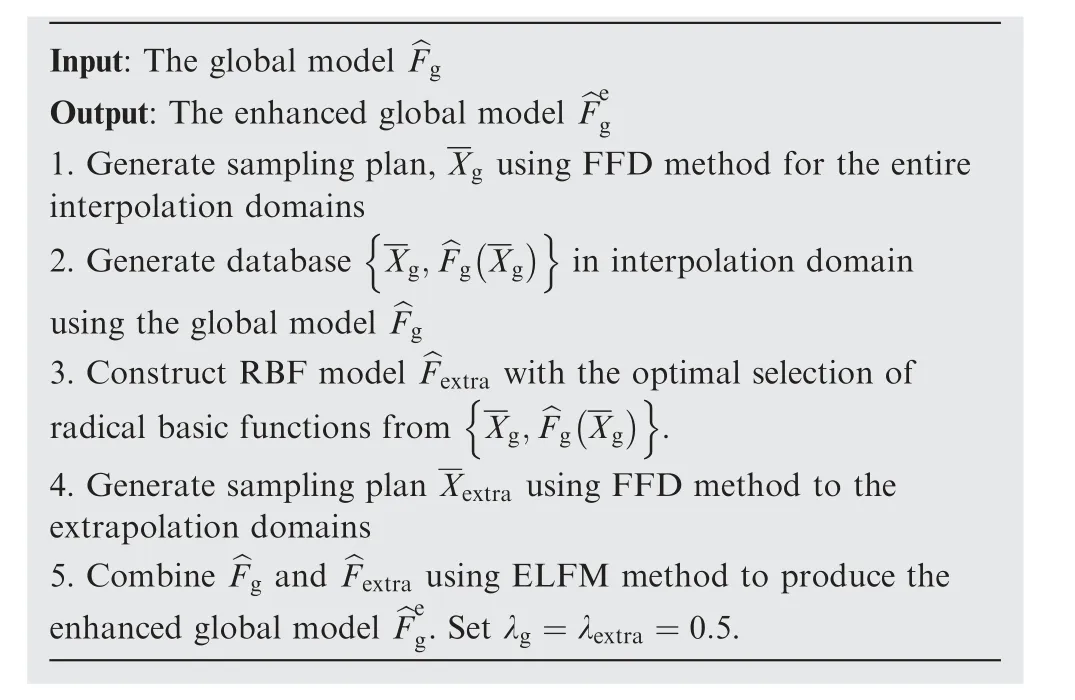
Algorithm 2 (Enhancing the global model for extrapolation).

4.Numerical experiments and analyses

In this section, several multi-dimensional analytical examples were used to verify the sequential modeling method of AMDF.Furthermore, an engineering case study of modeling an aerodynamic database of high-speed aircraft was used to illustrate the merits and effectiveness of the AMDF model, by comparing it with conventional approaches using Kriging, ECK, and LRMFS.The Relative Root Mean Square Error (RRMSE)and Relative Maximum Absolute Error (RMAE) are adopted to verify the surrogate model’s global and local accuracy,respectively15.The smaller the RRMSE and RMAE,the more accurate the model is.The expressions of both metrics are:

where ntestis the total number of the testing points, ^yiis the predicted response of the testing points,yiis the true response of the testing points, and yi and STD are the mean and standard deviation of all testing points, respectively.

4.1.A one-dimensional analytical problem

4.1.1.A pedagogical example

After the selection of surrogate models,Fig.9(a)shows the local models,which were constructed to in Eq.(8).The fidelity weights of f1(x ）,f2(x ）and f3(x ）are λ1=λ2=λHF=0.9 and λ3=λLF2=0.05, respectively.Fig.9(b) demonstrates the behavior of the weight functions of local models in different locations.In locations where the values of a specific weight function are equal to 1, the global AMDF model strictly follows the corresponding local model in its local domain.In locations where the weight values equal 0, the corresponding local model has no influence on the global model.The resulting global AMDF model is presented by the solid purple line in Fig.9(c).In the same figure, the global AMDF model is compared with other global models using conventional methods:the global Kriging model (green dashed line) was built with HF samples alone; the global ECK model (blue dash-dotted line) was built with all samples of LF1, LF2and HF datasets;the global LFMFS model (black loosely dashed line) was also built with samples from all datasets.All global models were validated with the HF testing samples (red crosses), and the absolute error between global models and the testing data is demonstrated in Fig.9(d).The accuracy investigation indicates that the AMDF model is significantly more accurate than other models in, both, the interpolation zone (x ∊[0,0.6])and the extrapolation zone (x ∊[0.6,1]) where there is an absence of HF data.Instead of extrapolating HF data, like other models, the global AMDF model follows the LF2data to maintain the tendency of the HF data.

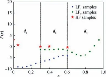
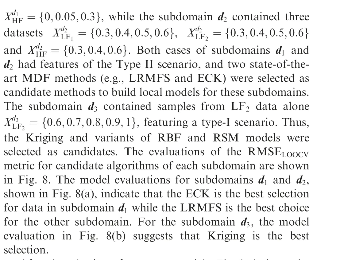
Fig.7 Distribution of sampling datasets and subdomains.

Fig.8 Model evaluations for different subdomains’candidate models by using metric RMSELOOCV.

Fig.9 Global model construction and accuracy comparisions.

To verify the accuracy of global models, 100 points were randomly selected.The accuracy results are shown in Table 3.An investigation was performed in different zones of the design space to verify the approximation capability of different global models.The accuracy analysis was performed at all local and global scales of the design space.For local scales,specifically in the interpolation region (x ∊[0,0.6]), both AMDF and LRMFS models showed outstanding accuracy compared to other models.The result is compatible with the error analysis results in Fig.9(d).However, in the extrapolation region (x ∊[0.6,1]), only the AMDF model still followed the tendency of HF testing point,while the other models failed to predict the tendency of HF data.That caused large errors in the prediction of Kriging, ECK and LRMFS models.This is because the kriging,ECK and LRMFS are interpolation methods and have less accuracy in extrapolation, while the AMDF used the available LF2data instead of performing an extrapolation.In this region, the LF2data still followed the tendency of the HF data.At a global scale, the accuracy analysis highlights the AMDF model as the most accurate model.

Table 3 Accuracy comparison of different approximation models.

In conclusion, the results of the accuracy analysis proved that the proposed AMDF is an appropriate approach for constructing global approximation models for multi-fidelity and non-uniform data.The AMDF model produced more accurate predictions than the conventional models with the same number of training samples.The AMDF model followed the highest fidelity data in local domains, which helped reduce the extrapolation work and satisfied a practical engineering sense.However,that is also the weak point of the AMDF framework if the LF datasets fail to reflect the trend of the HF dataset.It is also a problem with the other conventional multi-fidelity surrogate modeling methods.

4.1.2.Effect of domain decomposition

In the proposed AMDF approach, the design space is divided into subdomains featuring uniform data structures, which is a significant aspect of the proposed AMDF method.Therefore,local models are separately constructed using the surrogate modeling methods selected throughout the model selection process.The domain decomposition is based on the boundaries of the distribution domains of the datasets.However,domain decomposition also results in dataset split.The illustrative example in Fig.9 highlights this problem.In particular,the set of HF samples (red stars) was split into two separate sets that were found in the subdomains [0, 0.3] and [0.3, 0.6],as shown in Fig.9(a).Two local HF models, f1and f2, were constructed using the LRMFS and ECK methods, respectively.Using the ELFM method, as illustrated in Fig.9(c),these local models were combined to produce a global model(solid pink line).It has been noted that the AMDF model accurately followed the trend of both local and global HF models.Furthermore, the error estimation in Fig.9(d) shows that the AMDF model outperformed other modeling approaches in reflecting information on the HF data in the subdomain [0, 0.6].

In conclusion, the proposed AMDF method has significantly enhanced the quality of model construction by employing domain decomposition.As a result, the proposed AMDF framework differs from the existing modeling methods in producing a surrogate model for multi-fidelity data featuring diverse data structures.

4.1.3.Effect of fidelity weight

According to the comprehensive results presented above on the 1D example, the proposed AMDF is very promising for modeling non-uniform multi-fidelity data.The fidelity weights, λ,have a significant impact on AMDF performance because they determine the prioritized datasets to be modeled.In other words, by using the fidelity weights, the fidelity levels of multi-fidelity datasets are quantified and included in the behavior of the resulting model.Using Gaussian-based weight functions, the AMDF model maintains the local characteristics of the HF model in the subdomains with the presence of HF points while transferring the shared global and local features of the LF model to the HF model in the subdomains without HF points.The behaviors of the weight functions were influenced by two factors: (A) the correlation between the LF and HF samples and (B) the fidelity weights.Fig.10 demonstrates an inquiry carried out to assess the effects of the fidelity weight on the behavior of the AMDF model and the weight functions.Fig.10(a) depicts the behavior of the AMDF models with different values of fidelity weights λHFand λLF.Fig.10(b) depicts the behavior of the weight functions of HF model,wHF(x ）, with different values of weights λHFNote that λLF=1-λHFand wLFx( ）=1-wHF(x ）.We used the testing functions Eq.(16) and Eq.(17) as the HF and LF models,respectively.Besides,five HF samples(red triangles)were generated in the subdomain[0,5],and 11 LF samples(blue dots)in the domain [0,1].An additional set of ten HF samples (pink stars) was used only for validating the prediction of the constructed AMDF model.The LHS was utilized in the sample selection process.

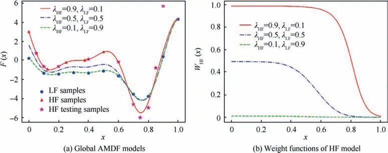
Fig.10 Impact of fidelity weights on behaviors of global AMDF model and HF weight function.

In the case of λHF=0.9,λLF=0.1, the information of HF samples is more important than the LF samples.The findings in Fig.10(a) demonstrate that the global AMDF model (solid red line)rigorously followed the local feature of HF samples in the subdomain [0, 0.5] and progressively transitioned to the local feature of LF samples in the subdomain [0.5,1] with no prior HF samples.In comparison to the HF testing results,the global feature HF samples were preserved in the subdomain[0.5,0.8].The values of wHF(x ）were near to 1 in the subdomain [0, 0.5] and progressively declined to 0 in the subdomain [0.5, 1) at the same time, as shown in Fig.10(b).

In the case of λHF=0.5,λLF=0.5,the roles of LF and HF samples are equivalent.The global AMDF(blue dash-dot line)followed the mean values of LF and HF samples in the subdomain[0,0.5].The wHF(x ）had a value of 0.5 in the corresponding subdomain,Fig.10(b).In the subdomain with no prior HF samples,the AMDF followed the local feature of LF samples,and the wHF(x ）was close to 0.

Finally,in the case of λHF=0.1,λLF=0.9,the information from LF samples is more important than the HF samples.In Fig.10(a),the global AMDF model(green dashed line)strictly followed the feature of the LF samples, and the values of wHF(x ）were close to 0 in the entire design space, as shown in Fig.10(b).In essence, the fidelity weights λ enabled the prosed AMDF to effectively extract the LF information during constructing the HF model.

4.2.Two-dimensional analytical problems

4.2.1.The Branin example

A comparison was performed between the proposed AMDF and three multi-fidelity approaches, including the ECK from Xiao et al.27,the LRMFS from Zhang et al.29,and the MFGP from Liu et al.41in the 2D Branin example41.Since there are only two levels of fidelity, the ECK becomes a similar form of the co-Kriging method from Kenedy and O’Hagan14.The two models of Branin function41with different fidelity levels were adopted for further investigations, shown in Fig.11.The expression of the high-fidelity function fHF(x ）and lowfidelity function fLF(x ）defined in D ∊[-5,10]× [0,15] are respectively given as:

Fig.11 HF and LF functions of Branin example.

The design space D0in Fig.11 was normalized to [0,1.0]2.In the subsequent investigation, we generated nLF=100 LF points in the domain [0,1.0]2, and nHF=20 partial HF points in the subdomain [0.5,1.0]× [0,1.0] using LH method.The response of fHF(x ）in the remaining region is more volatile and harder to predict41.Furthermore,the nHFwas varied from 10 to 30 to investigate the effect of HF training size on the modeling performance.For each case, 100 random runs were repeated to eliminate the influence of the design of experiments.To validate the model accuracy,5000 additional testing points were utilized to estimate the RRMSE of the resulting HF models using the four modeling methods.

Fig.12 depicts the boxplots of the RRMSE values of four resulting models with 20 partial HF points in the subdomain[0.5,1.0]× [0,1.0].The top line and the bottom line of the box represent the third quartile and the first quartile values,respectively.The lines inside the boxes represent the median values of the datasets and the markers (triangle, square, dot,diamond)denote the averaged values.The two horizontal lines outside the box represent the smallest and largest data points excluding any outliers,respectively.The red‘‘+”symbols represent the outliers.The results in Fig.13 indicate that the extrapolation of HF data in the subdomain[0.5,1.0]× [0,1.0] without prior HF data points is a nontrivial task to all the modeling methods.Particularly, the ECK and LRMFS models failed to provide reliable extrapolations of fHF.The lack of HF points posed a considerable challenge for the ECK and LFMFS in building a reliable discrepancy model in that subdomain.On the other hand,the MFGP and AMDF models, which saw a similar performance and higher levels of accuracy over the ECK and LFMFS.The MFGP used multiple Bayesian discrepancy models to transfer the shared global and local features of fLFto support the extrapolation of fHFin the subdomain[0.5,1.0]× [0,1.0].

Instead of extrapolating HF data in the subdomain[0.5,1.0]× [0,1.0], the proposed AMDF adopted distinct Gaussian-based weight models to directly transfer the global and local features of fLFto the prediction of fHF.In comparison to the MFGP, the proposed method lessened the computational costs and the impact of the distribution of HF points on the accuracy of the global model,yielding promising results Fig.12 (a).In addition, as shown in Fig.13, the AMDF captured the correct trend of fHFin the subdomain[0.5,1.0]× [0,1.0] with no prior HF data and outperformed the MFGP slightly in terms of RRMSE.That explains why in 100 repeating examples, the AMDF achieved better converged accuracy than the MFGP.Additionally, Fig.12 (b)investigates the impact of nHFon the performance of various modeling methods by using Branin example.It was observed that the AMDF and MFGP models generally had improvements in accordance with the increase of nHF.The AMDF showed the best performance among modeling methods.Conversely, the performance of the ECK and LRMFS declined as nHFincreased.

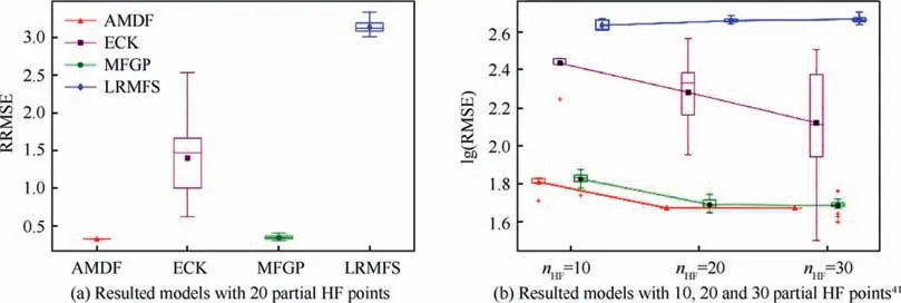
Fig.12 RRMSE values of four modeling methods over 100 runs on Brainin example with partial HF points in [0.5,1.0]× [0,1.0].

Fig.13 Demonstrative example of resulted models for Branin example with 20 partial HF points.

Finally, Fig.14 illustrates the behavior of the HF model’s weight function, wHF(x ）, in the design space in the case of 20 partial HF points.The characteristic of wHF(x ）was consistent over the 100 repetitive cases.It was observed in the subdomain[0.5, 1.0] × [0,1.0] that the AMDF assigned a wHFvalue close to 1, the AMDF model used the local feature of fHF.On the contrary, in the subdomain [0, 0.5] × [0,1.0], the wHFvalue was close to 0 in most runs, the AMDF model adopted the local feature of fLF.

4.2.2.Extrapolation example

In the 2D case,a two-variable function28was chosen to test the accuracy of the proposed framework in extrapolation problems with a single level of fidelity data.The expression of this function is defined as follows:

Fig.14 Demonstration of HF weight function in Branin example with 20 partial HF points in [0.5,1.0] × [0,1.0].

Two sampling plans, containing 14 points and 57 points,were chosen using the LHS method within the scope of the two variables:training samples(red triangles)and testing samples (purple stars), respectively.The distribution of sampling points is shown in Fig.15(a).In this example, the problem was constructing a global approximation model for the whole design space from a single training dataset.Firstly,a surrogate model was constructed for the interpolation region x1,x2∊[-2,0.8] where training samples existed.According to the steps of the AMDF framework, the RSM model with third order (RSM-3) was found to be an optimal selection to construct the interpolation model for the distribution domain of the training dataset.Fig.15(b) illustrates the prediction of the RSM-3 model in both the inner and outer sampling subdomains.However, the RSM-3 model saw an inaccurate prediction in the extrapolation region compared to the test data.To enhance the extrapolation capability of the resulting model, it was found that an RBF-cubic model is the optimal selection to construct an extrapolation model, as shown in Fig.15(c).The extrapolation model was constructed to clone the RSM- 3 model in the interpolation regions.Then, both two models were integrated into the global AMDF model, as shown in Fig.15(d).An accuracy comparison for different approximation models is shown in Fig.16.Different RBF models were constructed to clone correct trend of the RSM-3 model.Thus,they had similar values of RRMSE with the RSM-3 model for interpolation.However, the extrapolation performances of RBF models are much better than the RSM-3model.In particular, the RBF-cubic model saw an outstanding performance with the lowest RRMSE of extrapolation.The resulting global AMDF model retained the accuracy of the RSM-3 model in the interpolation subdomain and that of the RBF-cubic model in the extrapolation subdomain.Hence, the global model achieved a maximum accuracy.

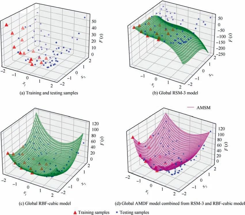
Fig.15 Global model construction in extrapolation scenarios.

Fig.16 Accuracy comparison of different approximation models for interpolation and extrapolation.

4.3.A six-dimensional analytical example

Next,the six-dimensional analytical example is used to test the performance of the proposed model.These functions are modified from Granacy and Lee.47The expressions of testing functions are given as:

In this six-dimensional example, we generated nLF=4096 LF points in the domain [0,1.0]6.The nhwas varied from 84 to 124 in the subdomain [0,0.5]× [0,1.0]5to investigate the effect of HF training size on the modeling performance.Similarly, the HF set had 20 repetitions for a comprehensive comparison.In addition,15000 test points were utilized to estimate the RRMSE of the HF forecasts made by using the four modeling methods.Fig.17 depicts the boxplots of the global and local accuracy of different models over the global domain[0,1.0]6using two accuracy metrics of RRMSE and RMAE,respectively.It was observed that the AMDF, MFGP, and LRMFS models generally performed better with the increase of nHF.

Conversely, the performance of the ECK declined as nHFincreased and had a significant volatility in all cases.Both the AMDF and LRMFS models saw quite similar values of accuracy metrics over 20 repetitions in each particular number of partial HF points.Even though the LRMFS is not often appropriate for non-uniform data, the accuracy of the LRMFS model outperformed the AMDF and MFGP in this example.

Fig.18 indicates the accuracy performances of different models in the interpolation subdomain [0,0.5]× [0,1.0]5.Note that the AMDF model also selected the LRMFS model to construct the local model of the HF data in the interpolation subdomain.Hence,the AMDF and LRMFS models were the best and had similar accuracy in the subdomain [0,0.5]× [0,1.0]5.It was concluded from previous discussion that the LRMFS model,with a good discrepancy model,captured the HF data’s tendency in the extrapolation subdomain [0.5,1.0]× [0,1.0]5.In contrast, the AMDF model purely followed the LF model in the extrapolation subdomain.Moreover, the LF model in this case did not capture the correct trend of the HF model in this subdomain compared to the LRMFS model.That could explain for the results in Fig.17 that the accuracy of the global LRMFS model was slightly higher than that of the AMDF model in the scale of the global domain.Indeed, the performance of the AMDF model is significantly dependent on the LF model’s accuracy in describing the HF model.The performance of the AMDF model can be reduced considerably if the LF datasets fail to describe the tendency of the HF data correctly.

The difference in the LRMFS model’s performances in the Branin and the six-dimensional examples makes it challenging to choose a dominant candidate or solution for modeling methods to deal with any data scenario.However, the results from the two mentioned examples proved the consistent performance and adaptability of the proposed AMDF approach when dealing with diverse data scenarios by producing highly accurate models compared to the ECK, MFGP, and LRMFS methods in the above experiments.

Fig.17 Accuracy comparisons of four modeling methods in domain [0,1.0]6 over 20 repeating runs in different numbers of partial HF points.

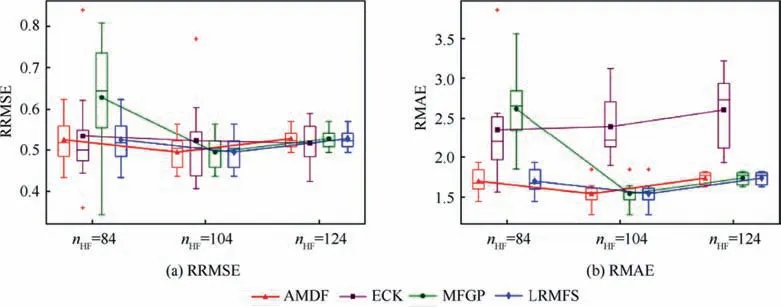
Fig.18 Accuracy comparisons of four modeling methods in interpolation subdomain [0,0.5]× [0,1.0]5 over 20 repeating runs in different numbers of partial HF points.

4.4.Engineering case: Generation of aerodynamic database for F16C fighter aircraft

In this work, the AMDF framework was implemented to model a database of the drag coefficient for a 1/15-scaled model of an F16C fighter aircraft in its different flight conditions.There were three independent variables:the Mach number, Ma, and the angle of attack, α, and the sideslip angle β.The range of variables were 0.1 ≤Ma ≤1.4, -20°≤α ≤50°,and 0°≤β ≤10°.The initial training data for the data fusion process was collected by performing three types of analysis with varying complexity, accuracy and computation resources required.

USAF Aircraft DATCOM (DATCOM)48is a computer program that calculates static stability, high-lift and control,as well as dynamic derivatives,using empirical methods developed in USAF.The program operates at a wide range of Mach numbers, as well as angles of attack higher than the linear region.In this research, DATCOM was treated as the lowfidelity analysis with the poorest prediction capabilities but wide operating range and fast calculations.

VSPAero (VSP)49is an open source, fast linear, vortexlattice method solver developed by NASA.In this research VSP is a low fidelity analysis method that is more accurate than DATCOM and valid only at linear regions.

ANSYS Fluent RANS CFD(CFD)solver is used as a highfidelity analysis tool.In this research, it produced the most accurate solution for the whole range of flight conditions.CFD is used to analyze both subsonic and transonic regions;the part of the database where other analysis methods fail.

The total number of the VSP sample points is ns1=370.The total number of the DATCOM sample points is ns2=400.And the CFD data is considered high-fidelity data,with ns3=54 points.Another set of 30 CFD samples was put aside as validation data.The values of fidelity weight for VSP, DATCOM and CFD datasets were assigned as 0.1, 0.1 and 0.8, respectively.Table 4 shows a setup of sampling plans for different analysis tools.

All the calculation cases were performed on a computer with an Intel Xeon E5-2680 v4 @2.40 GHz configuration and 128 GB of RAM.The computation cost of both VSP and DATCOM cases was a couple of hours.However,it took about 20 h per CFD case.Fig.19 shows a 1/15-scaled model of an F16C fighter aircraft.An unstructured mesh with 10970498 cells was applied for the CFD model.The current training data consisted of three datasets with different levels of fidelity and non-uniform distribution.Fig.20(a) illustrates a 2Dprojected view of training datasets’distributions when β=0°and varying α and Ma.The primary data domain was decomposed into subdomains in accordance with the boundaries of the datasets, as shown in Fig.20(b).In the next step, a surrogate model selection process was used to choose the best model type to approximate data in the subdomains.In this case, the subdomains d3and d4were subdomains containing samples from only one dataset, as S1and S2, respectively.Since the samples in subdomains d3and d4were from different sources and there is a small gap between two subdomains, the sampling data from both subdomains could be merged into a single dataset.Table 5 shows the selections of the surrogate models for each subdomain.

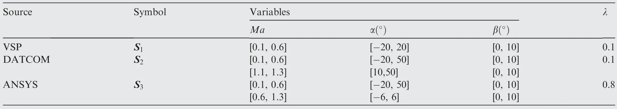
Table 4 Domains and analysis methods for drag coefficient computation.

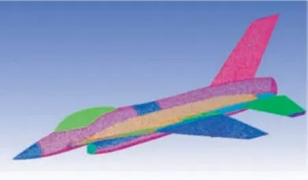
Fig.19 1/15-scaled model of F16C fighter aircraft.

After the local models for subdomains were constructed with the best choices of model types, the ELFM method was applied to combine all local models into a single global model.Then,an initial database with a total of 1200 points was interpolated in the inner zones of subdomains d1,d2,d3and d4.The interpolated database was used to construct a support model in the extrapolation enhancement process of the global model.The RBF-cubic model was selected as the support for the enhancement.Finally, a final global model was produced,which could perform interpolation and extrapolation everywhere in the design space.

Fig.21 shows various prediction models for the drag coefficient database in 2D surfaces when β=0°.The Kriging model was built with the CFD dataset (squares points) alone;the LRMFS and AMDF models used the CFD samples as HF datasets and VSP (dots) and DATCOM(triangles) samples as LF datasets, as shown in Fig.21(a), Fig.21(b) and Fig.21(c),respectively.For an intuitive representation, featured slices of three models in Fig.21(a), Fig.21(b) and Fig.21(c) were extracted at the same values of α=30°,β=0°and varying values of Ma and then presented in the same figure, as shown in Fig.21(d).It was observed that the AMDF model performed well in both interpolation and extrapolation of threedimensional domains.The Kriging and LRMFS models saw a low accuracy extrapolation compared to the validation data.

A comparison of the numerical accuracy of different global models, concerning interpolation and extrapolation performance, is shown in Fig.22.The AMDF model saw a greater accuracy than both Kriging and LRMFS models in interpolation and extrapolation regions.The accuracy metric RRMSE for interpolation was improved by 49% and 15% comparedto Kriging and LRMFS, respectively.With respect to extrapolation, the improvement was 79% and 56% compared to Kriging and LRMFS, respectively.

Table 5 Model selection of subdomains.

An additional investigation, shown in Fig.23, checked the extrapolation results of the investigated models, which followed the tendency of the target data.The validation data responses are plotted against the corresponding predicted values obtained by different methods.The points denoted by triangles are for conventional kriging that used CFD points alone, while the points denoted by stars and dots are for LRMFS and AMDF, respectively.The shorter the distance between the points and the line, the more accurate the model is.

The AMDF’s extrapolated results are, notably, in better agreement with the tendency of the validation data rather than Kriging and LRMFS.The Kriging and LRMFS are interpolation models based on an inverse correlation of Euclidean distance between the predictive location and training points.Hence, these models have less knowledge of predictive points outside the training dataset’s distribution domains.In this case, the Kriging and LRMFM failed to predict untried CFD data outside the distribution domain.The AMDF model did not try to extrapolate CFD data heavily.Instead, it used directly available DATCOM data in the local subdomain and only performed extrapolation in void regions using the RBF-cubic model.This practical strategy helped the AMDF model use the advantages of the component models in different data structures.However, this is also a weak point of the strategy when the DATCOM data needs to reflect the significant tendency of the CFD data correctly.The problem is the same as other conventional multi-fidelity surrogate models.In conclusion,the comparison shows the advantage of the proposed framework to achieve a complete solution for data fusion problems with multi-fidelity data with non-uniform structures.These are extremely difficult when using conventional approaches.

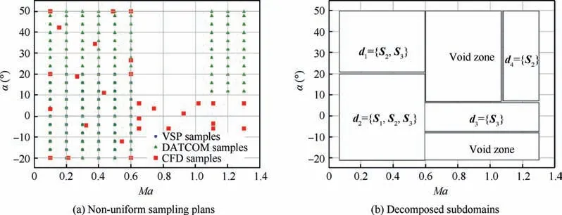
Fig.20 Initial sampling plans and subdomains of training datasets in a projected view at β=0° and varying α and Ma.

Fig.21 Comparison of different global approximation models of drag coefficient when β=0°.

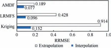
Fig.22 Accuracy comparison of different global models, modeling the drag coefficient in interpolation and extrapolation regions.

5.Discussion

Fig.23 True response and extrapolated responses of validation points.The straight line represents true response being equal to predicted response.

Although the performance of the proposed model was proved to be efficient for diverse data scenarios (i.e., multi-fidelity,multi-dimension,non-uniform data structures),the incorporation of multiple modeling methods in different subdomains and the selection of the modeling methods have some levels of computational complexity.The computational complexity of the proposed AMDF depends on that of the supporting models and the number of local models.Firstly, the computational complexity of the modeling process relies on the inversion of the covariance matrix and the dimensionality (i.e.,the number of hyperparameters)50.The proposed approach adopts different modeling methods to construct local models regarding the characteristics of the training data.The increase in the number of training data points increases the size of the covariance matrix.Moreover, a large number of dimensionalities makes the estimation of hyper-parameters a non-trivial high-dimensional optimization task.For the single-output multi-fidelity models, the computational complexity is O(n3）50and Q separate MF models can be constructed in the multi-output scenarios.Secondly, compared to conventional approaches, an additional computation cost is needed in the proposed AMDF for the selection process of modeling methods.However, the additional computational cost can be tolerated compared to the expensive simulations.

From analytical and engineering examples, the proposed AMDF approach is capable of dealing with highdimensional data fusion problems with high accuracy.This capability can be improved by constantly adopting novel modeling methods in the selection pool.The computational cost can significantly improve when fast modeling algorithms are incorporated.For engineering applications,most flight simulation applications adopt aerodynamic databases from two to three dimensions2,51,52; the proposed approach is promising for problems of aerodynamic database construction featuring intensive size, non-uniform data structures.As part of future work, an AI-based model selection process will be incorporated with the proposed AMFD framework for a short proposal of optimal candidates based on the characteristics of the input data.That is promising to reduce the number of model candidates to be evaluated in the model selection process, resulting in a significant reduction in the computational cost of the proposed AMDF’s modeling process.

6.Conclusions

This research proposes the AMDF framework as an automated process to efficiently solve data fusion problems with multi-fidelity data featuring non-uniform structures.In cases of uniform data structures, the AMDF framework resembles conventional approaches.Hence,the proposed AMDF framework can be applied to handle diverse scenarios of data fusion problems and data structures.The proposed approach was compared with four other modeling approaches (Kriging,ECK,LRMFS,MFGP models)through four analytical examples and an engineering example.

According to the comparison results,some conclusions can be drawn as follows:

(1) The proposed framework is capable of dealing with data fusion problems featuring multi-fidelity and multidimensional data and diverse data structures.The issues of interpolation and extrapolation are taken into account in the global model construction.

(2) The proposed framework uses flexible and practical strategy to efficiently utilize the advantages of the incorporated modeling methods in constructing accurate models, thanks to the model selection based on the features of training data.

(3) The adaptability of the proposed framework allows unlimited improvement and extension by updating new state-of-the-art modeling methods in the selection pool regardless of the algorithm of the individual modeling method.

(4) The engineering case, the accuracy metric RRMSE for interpolation of the CDis reduced by 49%, 15% using the AMDF model compared with that of the Kriging and LRMFS models.For the extrapolation of the CD,the reductions of RRMSE are 79% and 56% using the AMDF model compared to that of the Kriging and LRMFS models, respectively.While the modeling cost can be ignored when compared with the expensive simulations in the simulation-based design problem.Therefore, it can be an appropriate approach to deal with problems of aerodynamic database construction in applications of optimization design and flight simulation.

Declaration of Competing Interest

The authors declare that they have no known competing financial interests or personal relationships that could have appeared to influence the work reported in this paper.

Acknowledgments

This research was supported by the Basic Science Research Program through the National Research Foundation of Korea (NRF), funded by the Ministry of Education(No.2020R1A6A1A03046811).This paper was also supported by Konkuk University Researcher Fund in 2021.