Modeling and Adaptive Neural Network Control for a Soft Robotic Arm With Prescribed Motion Constraints

Yan Yang,Jiangtao Han,Zhijie Liu,,Zhijia Zhao,,and Keum-Shik Hong,

Abstract—This paper presents a dynamic model and performance constraint control of a line-driven soft robotic arm.The dynamics model of the soft robotic armis established by combining the screw theory and the Cosserat theory.The unmodeled dynamics of the system are considered,and an adaptive neural network controller is designed using the back stepping method and radial basis function neural network.The stability of the closed-loop system and the boundedness of the tracking error are verified using Lyapunov theory.The simulation results show that our approach is a good solution to the motion constraint problem of the line-driven soft robotic arm.

I.INTRODUCTION

FOCUSED on studies concerning the control of small deformation materials [1]–[5] and inspired by soft natural creatures,soft robotic arms [6] have been made by researchers to cope with unstructured environments in a variety of applications [7]–[9].Soft robotic arms can be driven in different ways,e.g.,fluid power [10],chemical reaction [11],and linedriven [12].For the line-driven soft robotic arm,the number and arrangement of lines can change depending on different scenes and functions to ensure that the soft armcan achieve different modes of motion and complete various tasks.A linedriven soft robotic arm has a faster response time than those of soft robotic arms driven by other approaches.Hence,the line-driven soft robotic arm should be further investigated.

The line-driven soft robotic armhas a flexible infinitedimensional feature,which is a challenging to model.At present,there are three commonly used methods to model soft robotic arms: finite element method modeling [13],piecewise constant curvature (PCC) method modeling [14],and Cosserat theory modeling [15],[16].The finite element method is used to solve the boundary value problem of a partial differential equation by decomposing an entire region into many simple subdomains (i.e.,finite elements).Thus,the solution domain is considered a minor,interconnected subdomain of many finite elements.Thereafter,it assumes a suitable approximate solution for each element and then derives an approximate solution for the entire problem[17].Although this method can be used in a variety of complex structures,it is difficult to obtain numerical solutions when applying internal or external motion constraints due to the calculation complexity.Therefore,researchers devised the PCC method as a plausible solution.Parameters,such as length,curvature,and deflection angle,can be used to describe the pose of the soft robotic arm in the PCC method,and the complexity of modeling is dramatically simplified [18].However,a PCC model can not cover all aspects of a soft robotic arm as it can only describe kinematics with fixed curvature.To obtain a more comprehensive description of soft robotic arms,the Cosserat theory was proposed in [19].A continuous Cosserat model is an infinitedegree-of-freedommodel,which assumes that soft robotic arms consist of infinite infinitesimal elements.These microelements are two-dimensional,such as the cross-section of a soft robotic arm,or one-dimensional like transverse fibers.The Cosserat method has been applied to the movement and operation of soft robotic arms [20].Although the accuracy of the model established by this method is high,the partial differential equations in this model cannot be effectively used for control design.In the usual Cosserat beam theory,the attitude matrix between individual sections exploits the Denavit-Hatenburg matrix in each local coordinate system,which may generate singularity;the screw theory can be used to model the entire system while avoiding this issue.In addition,the three-dimensional motion of a soft robotic arm is highly consistent with the screw motion.Therefore,we turned our attention to the screw theory because it can describe the motion of a soft robotic arm as a whole and simplify the complexity of the Cosserat rod.Adopting the above working methods,we inherit the ideal geometric and mechanical characteristics of the Cosserat model,such as inherent parameterization and significant general characteristics,describe a complete Cosserat rod using the screw theory,and combine it with the piecewise discretization method to design an accurate and precise model.

Control design for soft robotic arms is another challenge.Several studies have bee conducted on accurately controlling soft robotic arms,such as adaptive control [21],robust control [22],neural network (NN) control [23].In [22] and [24],a robust controller was designed for a soft robot armdescribed by the Cosserat rod.To avoid a sharp change in the actuating tension,the control input saturation was considered in the control design,and the effectiveness was demonstrated through the experiment and simulation.In [25],position/force hybrid control without force sensors was realized using the Cosserat theory and numerical calculation of the transformation matrix.In [26],an adaptive NN control was proposed for a soft robotic arm with external interferences and unmodeled dynamics.The stability of the closed-loop system and the convergence of the signal in the system were proved with Lyapunov function theory,ensuring that the end of the manipulator could track the given signal.However,the control methods for the soft arms mentioned above were real-time feedback control,which could not be implemented in a real application,and the asymptotic behavior of the closed-loop system was achieved without guarantee of the transient behaviors.

Constraints of transient behaviors are regarded as a key topic in the control of soft robotic arms in an unstructured limited environment.Barrier Lyapunov functions (BLFs) are skillfully constructed to deal with motion constraints [27]–[31].The constraints on the states or outputs of the systems in[27]–[31] are constants,therefore time-varying BLFs are proposed in [32] and [33].In [32],an asymmetric barrier Lyapunov function (ABLF) based on finite-time adaptive NN control was presented for a class of nonlinear strict feedback systems.The ABLFs were designed to deal with the timevarying asymmetrical full state constraints.An NN-based adaptive fault-tolerant control with BLF was used to make the tracking error satisfy the prescribed performance in the presence of actuator failures in [33].In this study,to ensure the accurate movement of the soft robotic arm,the time-varying BLF based control will be designed for the soft robotic armto guarantee the steady and the transient motion performance.

Motivated by the above discussion,this paper presents a dynamic model and adaptive NN control for a line-driven soft robotic arm.The dynamics model of the soft robotic armis established using the screw and Cosserat theories.An adaptive NN controller is designed to realize the trajectory tracking.Besides,considering the high precision control of the soft robotic arm,the time-varying BLF is designed to deal with the motion constraints.The main contributions of this study are as follows:

1) When incorporating the screw theory into modeling a soft robotic arm,the screw theory is employed to describe the motion of the soft robotic arm as a whole,prevent the singularity caused by the use of local coordinate system,describe the motion clearly,avoid the disadvantages of abstract mathematical symbols,and simplify the analysis of the Cosserat rod.

2) In practice,measurement error and unknown perturbations are unavoidable.Thus,the measurement error between strain state and speed,and unknown perturbations are considered.An adaptive feedback controller based on NNs is designed to deal with both parametric and nonpara-metric uncertainties caused by the measurement error and unknown perturbations including the unmodeled dynamics and external disturbances.

3) The spatial movement constraints of the soft robotic arms and the imposed performance function are deftly transformed into pose-tracking error bounds.Consequently,an adaptive NN control is designed for the soft robotic arm to track the desired trajectory and ensure that the tracking error cannot violate the prescribed motion constraints no matter whether the uncertainties exist or not.

Notations: SE(3) represents a three-dimensional Euclidean group that is the set of transformmatrices,S O(3) represents a three-dimensional orthogonal group,andso(3) andse(3) are lie algebras corresponding toS O(3) andS E(3),respectively.

II.DYNAMICAL MODEL OF A SOFT MANIPULATOR SYSTEM

A.Continuous Dynamics

Lie group theory is used to explain the deformation of the continuous Cosserat model [34].The Cosserat rod consists of many points.At a certain moment,the position of each point with respect to the basic frame is uniquely determined by a position vectorp(χ,t) and a rotation matrixT(χ,t),with χ ∈[0,L],whereχdenotes each point on the soft arm,Lis the overall length.Thus,the location functiong(χ,t)∈S E(3) used to define every point of the soft arm

Defineras the soft arm’s strain state that is expressed as

wherer=r(χ,t)is the strain state.rconsists of the angular strainsqand linear strainslrepresented asse(3),whereis the isomorphism between the vector representation and the matrix representation of the Lie algebrase(3).Furthermore,it can be represented asr=[q;l]∈R6,whereq(χ,t)∈R3represents the angular strains andl∈R3denotes the linear strains.

Fig.1.Soft armmotion model.

The following formula is employed to measure the spatial position derivative with respect toχ:

The derivative of spatial position to the timetis determined as

Then,b′can be calculated using (4)−(6) as

whereadr=[[q×],0;[l×],[q×]].The acceleration is calculated through differentiating (7) as

The screwPis described using the kinetic screw theory as

Invoking (9),the continuous dynamics is obtained as follows:

An internal elastic forceFi∈se(3)∗can be drawn based on the Kelvin-Voigt viscoelasticity theory as

whereKs=diag{GJx,EJy,EJz,EA,GA,GA} is the stiffness matrix,Kv=diag{Jx,3Jy,3Jz,3A,A,A}µvis the viscosity matrix;E,G,and µvare Young’smodulus,shear modulus,and shear viscositymodulus,respectively;r∗=[0 0 01 0 0]Trepresents the zero strain vector in the reference straight coordinates.

The adjoint representation (Ad) of Lie groupS E(3) is introduced in the preceding derivation,which is specified as (along with the coadjoint mapA d∗)

B.Piece-Wise Discrete Dynamics

The continuous dynamic model should be converted into a discrete dynamic model to improve the computational efficiency.The transformation is performed using the discrete segmental method.As shown in Fig.2,at any timet,the soft armcan be discretized intoNsegments,and the strain in each section can be specified withr n,n∈{1,2,...,N}.

Fig.2.Sketch of soft arm model.

Remark 2:Using the discrete segmental method,we can convert the partial differential equations into a homogeneous linear ordinary differential equation (ODE).For example,using the strain screwrn,n∈{1,2,...,N},(5) becomes a homogeneous linear ODE and the analytic solution can be obtained.The soft arm is divided intoNsegments,χ ∈[(0,L1),(L1,L2),(L2,L3),...,(LN−1,LN)],L=LN,and the initial value of segmentnwill be the right boundary condition of the segmentn−1 (χ=ln−1).

Then,(5) becomes a homogeneous linear differential equation.By integrating (5),we obtain

According to the exponential mapping theory [35],(13) is written as

Similarly,by integrating (8),we have

According to the properties of adjoint mapping of the Lie group,(20) is expressed as

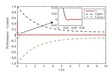
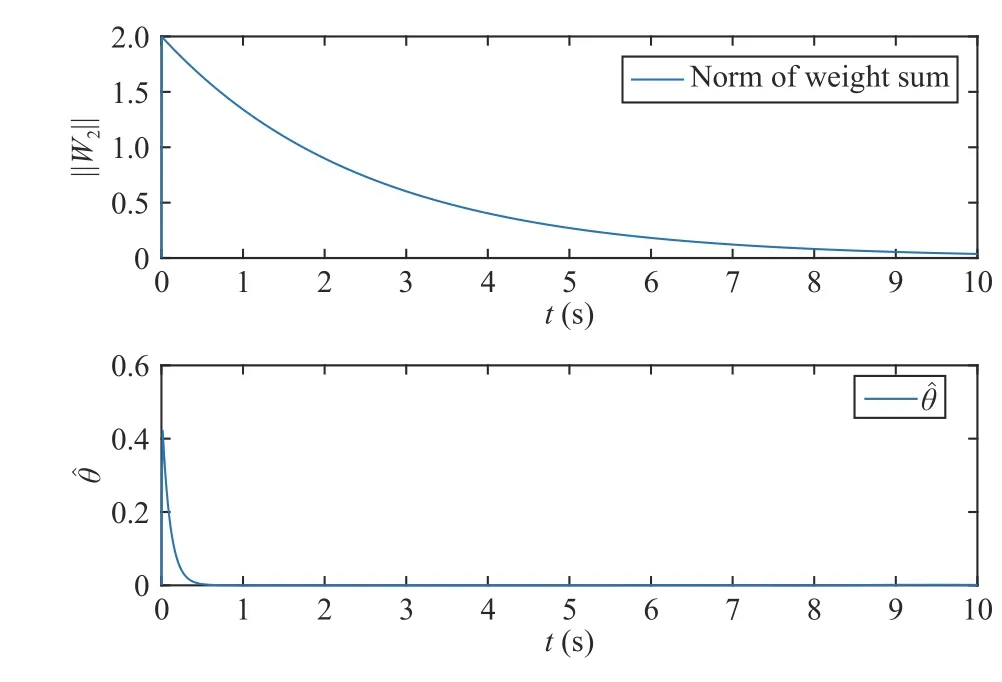
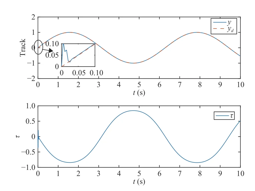
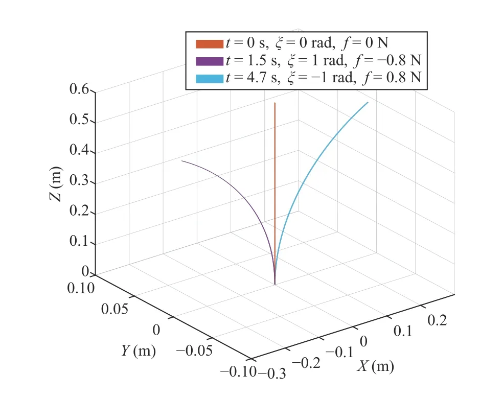
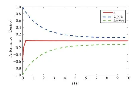
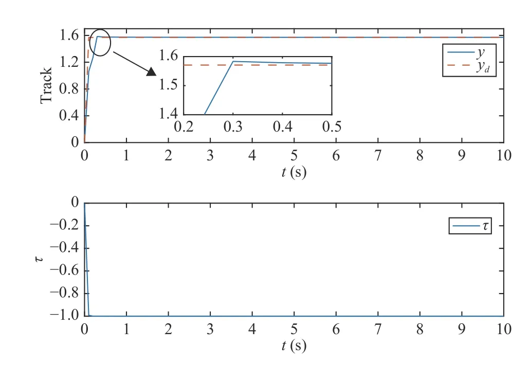
whereJ(χ) is the soft armgeometric Jacobian matrix,jis the descending index,Ln−1<χ

The Jacobian matrix has the following forms:

Given that the strainrnis known,Ad(gn) andAD(gn) can be calculated.Subsequently,the Jacobian matrixJ(χ) is calculated.The accelerationis derived as

where

Remark 4:The weak form of the partial differential equation can be derived by the extended Poincare variational method [34].The purpose of transforming the differential equation into a weak formis to reduce the requirements for the partial differential equation solution,which ensures that the solution of the equation exists in a discrete form.The weak formcan reduce the requirement for the continuity of the solution of the equation.Therefore,the continuous dynamic model can be transformed into a piecewise discrete model.

Substituting (22) and (24) into (26),we obtain

Furthermore,we obtain the discrete dynamic model using the following equation:

and τi,i=1,2,...,nis expressed in the following form:

We assume that the elastic and actuation loads are along the section,that is,F a(Ln−1<χ

whereFanis the internal drive load of the cables atLn,Finis the internal load atLn.

Substituting (32) into (31),we obtain

Thus,the dynamic model is written as

III.PRELIMINARIES AND PROBLEM FORMULATION

A.Model Transformation

For the subsequent control design,we transform the model into a sate space equation.τnis described by (33),and divided into two segments,i.e.,elastic and actuation loads;hence,τcan be written as τn=τi+τa,and the tension of the cable can be separated.

The tensionFai∈R6can be expressed as

whereFixm,Fiym,andFizmrepresent the moment applied on theX,Y,andZaxes,respectively.Similarly,Fix,Fiy,andFizare the forces applied onX,Y,andZdirections,respectively.

B.State Space Equation

whereU(x1) is an unknown and continuous function involving both parametric and nonparametric uncertainties caused by measurement errors;f=M−1(D+U(x1,x2)) is an unknown termcomposed of generalized inertialM,the unknown internal perturbationD,and the uncertaintiesU(x1,x2).

Assumption 3: xd=[xd1,xd2,...,xdn] is a continuous and 2nd order derivative tracking signal.We assume thatxdis bounded and satisfies ∥xd(i)∥≤xdc,wherexdcis a positive constant.

C.Neural Networks

Radial basis function neural network (RBFNN) can be introduced as follows:

whereZ=[Z1,...,Zp]T∈ΩZ⊂Rp,H∈Rς,hiis theith weight,andsi(Z) has the following form:

where ℑiis the width of the Gaussian function and κiis theith hidden node’s center.Then,the RBFNN can approximate Ψ(Z)with arbitrary precision,which is expressed as

whereH∗Tis an ideal constant weight vector,and ϵ(Z) is an approximation error with |ϵ(Z)|≤ϵ,whereϵis a positive constant.

Lemma 2:To enable the systemto achieve the specified performance,a BLF is utilized

where ln(·) represents the natural logarithm andais the performance function.In the set |z|

Lemma 3:If |b|<1,then the following formula holds:

Remark 5:The prescribed performance function F is selected as

where ι>0 and F0>F∞>0,andFsatisfies F(0)=F0and limt→+∞F(t)=F∞,then the prescribed performance of the tracking errorz1=y−yrcan be ensured.

IV.CONTROL DESIGN

The control objective in this paper is to design an adaptive NN control such that the soft robotic arm can track the desired trajectory and ensure that the tracking error cannot violate the motion constraints.

The soft arm moves within the specified range,and the system meets the predetermined performance,if the norm of the tracking error satisfies the following inequality:

where Θ>0 is an adjustable constant,ΘF0represents the upper bound of the maximum allowable overshoot,and Θ F∞represents the allowable upper bound of the steady-state tracking error.

Based on the above properties,a time-varying BLF is designed to fulfill the predefined tracking error constraint.Define the following function as:

with

Remark 6:Owing to the properties of the Gaussian function,the following formula is obtained:

whereldis the number of NN nodes.

Remark 7:There exists a positive constantsuch that the following inequality holds:

whereI∈Rn×nis t he identity matrix.

According to (47) and (50),ξis defined as

Thus,the time-varying BLF candidateV1is rewritten as

The barrier function should be set appropriately to meet∥z1(0)∥

The block diagram for the proposed control is as shown in Fig.3,and the proposed control scheme is summarized in Table I.Then,we give the following theorem.

Fig.3.The control block diagram.

Theorem 1:Considering the soft robotic arm(40) under Assumptions 1−4,using the proposed control schemes (64)and (74) and the adaptive law s (65) and (75),the following properties hold: 1) all signals in the closed-loop system are bounded and 2) the norm of tracking error ||z1|| satisfies the prescribed motion constraint (47).

Proof:Choose the following Lyapunov function:

According to Lemma 3,we obtain

TABLE I ADAPTIVE NEURAL NETWORK CONTROL SCHEME FOR A SOFT ROBOTIC ARM

V.NUMERICAL SIMULATION

In this section,two examples are provided to illustrate the effectiveness of the proposed controller.We assume that the axial strain in they-axis andz-axis directions is ignored.The physical parameters of the soft robotic armare provided in Table II.

In the simulation,the initial values are selected asx(0)=[0;0;0;0.5;0;0],andr∗==[0;0;0;0;0;0].The time-varying signal is selected asxd(1)=[0;sin(t);0;0;0;0],and the step signal is chosen asxd(2)=[0;π/2;0;0;0;0];We choosef=[0;sin(r2);0;0;0]Twith the boundary of the unknown function=[1;1;1;1;1;1]T.The parameters of the controller are provided as follows:F0=1,F∞=0.1,ι=0.6,δ1=2,δ2=1,Γ1=0.2,Γ2=1,Θ=1,K1=800,andK2=800.

Remark 8:The influence of the parameters (ι,F0,F∞,k1,k2)on the control performance is explained.ιaffects the decay speed of the performance function,and the decay rateincreases withι.F0affects the initial value of the performance function.F0should be larger than the initial value of tracking errors.The value of F∞affects the steady state error of the system.The closed-loop performance can be optimized by increasing the values ofk1andk2.However,improper values may cause the instability of the system.

TABLE II PARAMETERS OF THE SOFT ROBOTIC ARM

Case A:Time-varying signal

In the first example,we consider the soft armtracking a time-varying signal.The simulation results are shown in Figs.4–7.In Fig.4,the blue dotted line represents the upper bound of the allowable error,which decreases with time to the maximumupper bound of the steady-state error;the green dotted line represents the allowable lower bound of the error,and the maximumlower bound allowed by the steady-state error is finally reached with time.Fig.5 shows the weight norm of the NN ∥W2∥ and the adaptive parameterθ.The control inputτand the trajectoryyare shown in Fig.6.We can see that with the proposed control,the soft arm can quickly track the time-varying signals after 0.06 s depicting the effectiveness of the proposed controller.Fig.7 is a three-dimensional model of a soft arm.The orange line represents the position of a soft arm when no force is applied,and the bending angle is 0 rad;the purple line represents the change in position of the softarmat 1.5 s when the applied force is–0.8 N and the bending angle is 1 rad;the sky blue line represents the change of the position of the softarmat 4.7 s when the applied force is 0.8 N and the bending angle is −1 rad.

Fig.4.Tracking error z1 with output constraints for Case A.

Fig.5.Parameter configuration for Case A.

Fig.6.Signal tracking performance and control input for Case A.

Case B:Step signal

In the second example,let the soft robotic armtrack a step signal.The simulation results are shown in Figs.8–10.In Fig.8,the blue dotted line represents the upper bound of the allowable error,the green dotted line represents the allowable lower bound of the error,and the red solid line represents the tracki ng errorz1.Fig.9 shows the weight norm of the NN∥W2∥and the adaptive parameterθ.The control inputτand the trajectoryyare shown in Fig.10.We can see that with the proposed control the soft armcan quickly track the step signal after 0.05 s.We can conclude that the soft armunder the proposed adaptive NN control scheme can track the desired trajectories and ensure that the tracking error cannot violate the prescribed motion constraints even in the presence of uncertainties.

Fig.7.Three-dimensional model with time-varying signal for Case A.

Fig.8.Tr acking error z1 with output constraints for Case B.

Fig.9.Parameters configuration for Case B.

VI.CONCLUSIONS

In this study,we presented a piece-wise discrete dynamic model of a line-driven soft robotic arm based on the screw theory and the Cosserat theory.An adaptive NN control scheme was proposed for the soft armto track the desired trajectory.The RBFNN was used to deal with the uncertainties including the measurement error,unmodeled dynamics,and external disturbances.Then,the time-varying BLF was designed to ensure that the tracking errors cannot violate the prescribed motion constraints.The numerical simulations verified the effectiveness of the presented control scheme.However,this study only uses theoretical analysis and numerical simulations to demonstrate the availability of the proposed control and an experimental demonstration will be undertaken in our future work.

Fig.10.Step signal tracking performance and control input for Case B.