RANSACs for 3D Rigid Registration:A Comparative Evaluation

Jiaqi Yang, Zhiqiang Huang, Siwen Quan, Zhiguo Cao, and Yanning Zhang,

Abstract—Estimating an accurate six-degree-of-freedom (6-DoF) pose from correspondences with outliers remains a critical issue to 3D rigid registration. Random sample consensus(RANSAC) and its variants are popular solutions to this problem.Although there have been a number of RANSAC-fashion estimators, two issues remain unsolved. First, it is unclear which estimator is more appropriate to a particular application. Second, the impacts of different sampling strategies, hypothesis generation methods, hypothesis evaluation metrics, and stop criteria on the overall estimators remain ambiguous. This work fills these gaps by first considering six existing RANSAC-fashion methods and then proposing eight variants for a comprehensive evaluation.The objective is to thoroughly compare estimators in the RANSAC family, and evaluate the effects of each key stage on the eventual 6-DoF pose estimation performance. Experiments have been carried out on four standard datasets with different application scenarios, data modalities, and nuisances. They provide us with input correspondence sets with a variety of inlier ratios, spatial distributions, and scales. Based on the experimental results,we summarize remarkable outcomes and valuable findings, so as to give practical instructions to real-world applications, and highlight current bottlenecks and potential solutions in this research realm.

I. INTRODUCTION

RIGID registration of 3D data (point clouds, meshes, or depth maps) aims at estimating an accurate six-degree-offreedom (6-DoF) pose to transform the source shape to the coordinate system of the target shape. It finds a number of real-world applications, such as 3D modeling [1]–[3], 3D object recognition [4], and localization [5].

At present, 3D registration methods can be classified as learning-based or non-learning-based. For learning-based methods [6]–[11], most try to solve the registration problem in an end-to-end fashion, such as DGR [7] and 3DRegNet [8].The experimental datasets of these methods are mainly synthetic model datasets, and their robustness to large-scale and real-world noisy data deserve further investigation. Besides,there are also some learning-based methods that learn a feature descriptor (such as 3DMatch [12] and PPFNet [13]) or a feature matcher (such as PointDSC [10]) first, and then employ traditional 6-DoF pose estimation modules to achieve registration. A practical issue for learning-based methods may be the lack of adequate training data in some real-world applications.

For non-learning based methods, a typical solution is searching consistent point-to-point correspondences between 3D shapes [14]–[17] (Fig. 1). Although three non-coplanar correct correspondences are sufficient to estimate a reasonable 6-DoF pose, the initial correspondences established by matching local geometric descriptors are usually contaminated by severe outliers due to the following reasons.i)Data nuisances.The raw point clouds captured by existing 3D sensors often contain noise with different scales. The variation of scanning viewpoints and distances will result in limited overlaps and point density variation, respectively. Furthermore,one should expect clutter and occlusion in complex scenes.ii)Keypoint localization errors.Existing keypoint detectors still exhibit limited repeatability [18]. Therefore, some truly corresponding points cannot be identified.iii)Limited robustness of local geometric descriptors.Most of the current local geometric descriptors are sensitive to partial overlap, occlusion, and repetitive patterns [19], while robust local shape description is critical to achieving consistent correspondences [20]. Therefore, the problem boils down to computing an accurate 6-DoF pose from a correspondence set with heavy outliers. Random sample consensus (RANSAC) [21] is a well-known solution to the robust 6-DoF estimation problem [22]. It repeatedly generates hypotheses by randomly sampling three or more correspondences and evaluates the quality of generated hypotheses based on the spatial consistency of correspondences. However, RANSAC suffers from two main limitations. First, the computational complexity of RANSAC isO(n3)and estimating a reasonable pose requires a huge number of iterations. Second, RANSAC generates hypotheses randomly and may fail to find the optimal solution, especially when the given correspondence set contains scarce inliers. To solve these problems, many variants of RANSAC have been proposed in the 3D vision realm [14], [23]–[26], which mainly modify RANSAC from three aspects.i) Reducing the theoretical computational complexity.This is typically achieved by leveraging point orientations, such as normal and local canonical frames, therefore only one or two samples (three or more for the standard RANSAC) are required for hypothesis generation per iteration. This can greatly reduce theoretical computational complexity.ii) Improving the quality of generated hypothesis.Before hypothesis generation, geometric constraints can be employed to rejectbadsamples, which can improve the overall quality of generated hypotheses.iii)Proposing different hypothesis evaluation metrics to find the optimal hypothesis.In addition to the inlier count metric, additional geometric cues, such as point distances and point cloud overlap information, are considered to improve the reliability of the hypothesis evaluation step. In addition to RANSACfashion methods, other non-learning-based methods include iterative closest point method (ICP) and its variants [27], gravitational methods [28], optimal transport methods [29], and probabilistic methods [30]. The readers are referred to a recent survey [31] for a comprehensive review.

Fig. 1. The objective of 6-DoF pose estimators is to compute an accurate 6-DoF pose comprised of a rotation matrix R ∈S O(3) and a translation vector t ∈R3for two 3D rigid shapes from a set of point-to-point correspondences with outliers. Black dots: keypoints; green lines: inliers (correct correspondences); red lines: outliers (false correspondences).

Related Evaluations:Although there have been a number of evaluations related to correspondence generation [18]–[20],evaluation efforts on 6-DoF pose estimation from correspondences are still limited. Yanget al. [14] evaluated the performance of OSAC and RANSAC on several groups of point clouds in the context of point cloud registration, and showed that OSAC achieves better precision performance than RANSAC. Guoet al. [17] compared the performance of consistent correspondences verification (CCV) and RANSAC on a 3D modeling benchmark; they demonstrated that CCV achieves higher registration precision than RANSAC and several of its variants with different numbers of iterations. Yanget al. [26] assessed the performance of RANSAC, GC1SAC,and 2SAC-GC when applied to aligning point cloud views with limited overlaps; they determined that 2SAC-GC achieves better performance than the other two competitors under a variety of iterations. Quanet al. [25] evaluated the performance of RANSAC and GC1SAC in terms of registering point clouds scanned by low-cost sensors; they revelaed that GC1SAC consistently outperforms RANSAC when performed on correspondences obtained by matching different local geometric descriptors. Recently, Zhaoet al. [32] conducted an evaluation of several 6-DoF pose estimators in terms of mismatch removal and 3D registration accuracy on four point cloud registration datasets.

Unfortunately, none of the above evaluations exhaustively tested the performance of 6-DoF pose estimators in the RANSAC family. First, only a few number of existing estimators are considered for comparison. Second, the evaluation datasets only address a particular application with limited nuisance types. Third, only the overall estimators are tested, and the effects of key stages in the RANSAC pipeline, such as sampling, hypothesis generation, hypothesis evaluation, stop criterion, have been overlooked.

Focus of This Evaluation:Since RANSAC has been proposed for nearly forty years, there have been a large number of RANSAC variants at present. They can be categorized into two classes: general estimators and task-specific estimators(the task refer to as 3D rigid registration in this paper). The former ones are independent from application scenarios, e.g.,MLESAC [33], LO-RANSAC [34], USAC [35], Graph-cut RANSAC [36], and MAGSAC++ [37]. The latter ones, e.g.,sample consensus initial alignment (SAC-IA) [24], 1-point RANSAC (GC1SAC) [23], optimized sample consensus(OSAC) [14], 2-point based sample consensus with global constraint (2SAC-GC) [26], global constrained 1 point-based sample consensus (GC1SAC) [25], particularly leverage some unique geometric properties of point clouds, such as normal and local reference frames (LRFs) [38], to improve registration accuracy and/or efficiency.

In this evaluation, we put our focus on the latter category(there are fourteen for evaluation). This is because point clouds provide rich geometric cues for RANSAC estimators,and comparing RANSAC variants in this category can more clearly reveal: 1) What kinds of geometric cues are reliable and appropriate for a particular application; 2) How to properly incorporate these geometric cues into RANSAC; 3) The effects of various point cloud geometric properties on registration accuracy and efficiency; 4) Specific future directions for mining other good geometric cues to further improve RANSACs’ registration performance. In addition, for the problem of 3D rigid registration, RANSAC-based methods are still worth a comprehensive evaluation because they have their own merits in various registration scenarios and deliver outstanding performance in both object and scene registration scenarios in recent publications [15], [39], [40].

Motivation and Contributions:Although a variety of registration methods have been proposed, we are motivated to evaluate the RANSAC-family methods due to the following reasons:

i) Theoretically efficient and robust:From a theoretical view, RANSACs are efficient because they operate on sparse correspondences rather than dense point clouds, and are robust because they follow a hypothesis-and-verify pipeline to achieve robustness to outliers. In addition, RANSACs do not need training data. By contrast, most other registration methods fail to achieve balanced performance. For instance,learned methods usually require massive training data; ICP methods tend to fall to a local minimum; probabilistic methods generally suffer from high computational complexity.

ii) Verified superior performance:Even in the deep learning era, RANSACs achieve competitive performance as compared with learning methods. Specifically, Baiet al. [10]recently demonstrated that RANSAC outperforms two end-toend learning methods, i.e., DGR [7] and 3DRegNet [8], and achieves comparable performance as a learning feature matcher method, i.e., PointDSC [10], in 3D scene registration scenario. In addition, we also compare RANSACs with four state-of-the-art using our experimental datasets and further verify the competitive performance of RANSACs.

iii) Easy to implement:RANSACs that iteratively perform hypothesis-and-verify have low implementation complexity,making them very popular in many fields (RANSAC now is available in several popular 3D vision open source libraries,such as OpenCV [41], PCL [42], and Open3D [43]).

iv) Great potential to be even better:As will be revealed by our evaluation, although existing RANSACs already achieve competitive 3D registration performance, they still hold great potential to be more efficient and robust by developing more advanced sampling strategies and hypothesis evaluation metrics.

v) The lack of a comprehensive evaluation:The performance of existing RANSACs remain unclear in the presence of different application contexts, because these estimators are usually evaluated on small-scale datasets and the comparison with state-of-the-art methods is not conclusive. Moreover,there is a lack of convincing evaluation methodologies and experiments to support the fair comparison of sampling strategies, hypothesis generation methods, hypothesis evaluation metrics, stop criteria, as well as overall estimators.

Motivated by these considerations, we give an evaluation of fourteen 6-DoF pose estimators in the RANSAC family. They include six existing methods, i.e., RANSAC [21], SAC-IA[24], GC1SAC [23], OSAC [14], 2SAC-GC [26], GC1SAC[25], as well as eight variants of RANSAC proposed in this evaluation.The objective of the proposed RANSAC variants is to particularly evaluate the effects of each key stage on pose estimation performance and fairly compare existing sampling strategies, hypothesis generation methods, hypothesis evaluation metrics, and stop criteria.To achieve a comprehensive evaluation, we deploy experiments on four standard datasets with different data modalities, application scenarios, and challenging configurations such as Gaussian noise, uniform data decimation, random decimation, holes, varying scales of input correspondences sets, and varying detector-descriptor combinations. This helps to generate correspondence sets with varying inlier ratios, spatial distributions, and scales. Our contributions are summarized as follows:

a) We perform a survey of six existing 6-DoF pose estimators in the RANSAC family and additionally propose eight RANSAC variants. An abstraction of the core ideas of these fourteen estimators and their key stages is given, in order to systematically compare the theoretical aspects of evaluated estimators and highlight their traits.

b) A comprehensive quantitative evaluation of fourteen 6-DoF pose estimators on datasets with different data modalities, application scenarios, and challenging configurations such as Gaussian noise, uniform data decimation, random decimation, holes, varying scales of input correspondences sets,and varying detector-descriptor combinations. The tested terms cover the main concerns for a 6-DoF pose estimator,i.e., accuracy, robustness to challenging experimental configurations, and efficiency.

c) A summary of remarkable experimental outcomes and valuable findings, in order to give practical instructions to real-world applications, and highlight current bottlenecks and potential solutions in this research realm.

Paper Organization:The rest of this paper is organized as follows. Section II presents an abstraction of the core ideas of the fourteen considered estimators and their key stages. Section III introduces the experimental datasets, evaluated terms,evaluation metrics, and implementation details. Section IV presents the experimental results where necessary discussions and explanations are given. Section V gives a summary of the peculiarities of evaluated methods. Finally, the conclusions are drawn in Section VI.

II. CONSIDERED 6-DOF POSE ESTIMATORS

All considered 6-DoF estimators in the RANSAC family consist of several common key stages, e.g., sampling, hypothesis generation, hypothesis evaluation, and stop criterion. To avoid redundancy, we abstract the core ideas of each key stage rather than introduce each estimator independently, because all considered estimators follow the pipeline depicted in Fig. 2. Then, our proposed RANSAC variants and the motivation behind are described.

Fig. 2. The general pipeline of 6-DoF pose estimators in the RANSAC family.

A. Key Stages of Considered Estimators

1) Sampling:Sampling strategies can be categorized asrandom samplingandconditional sampling. The latter usually leverages geometric constraints to find more convincing samples.

Random sampling (RS):A straightforward sampling manner is randomly choosing one, two, or three correspondences from the correspondence set C (i.e., 1-point, 2-point, and 3-point sampling strategies, respectively). A pose hypothesis can be generated with three non-coplanar correspondences if using the coordinate information of the associated keypoints of correspondences only; two non-collinear correspondences are sufficient if a canonical orientation (e.g., the normal vector) is available at each keypoint; one correspondence is enough if an LRF is constructed for each keypoint. For instance, RANSAC and GC1SAC randomly select three candidates and one candidate per iteration, respectively.

Conditional sampling (CS):There exist two approaches in this category.

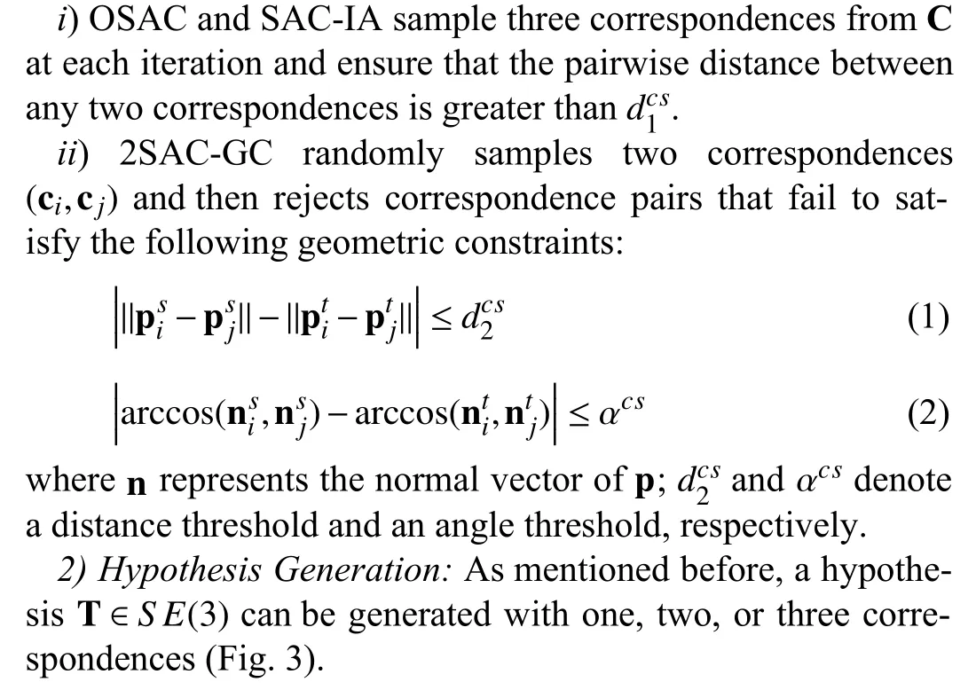
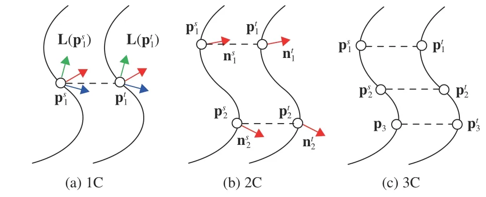
Fig. 3. A 6-DoF pose hypothesis can be generated with one (1C), two (2C),or three (3C) correspondences. Here, p, n, and L denote a 3D keypoint, a normal vector, and an LRF, respectively.

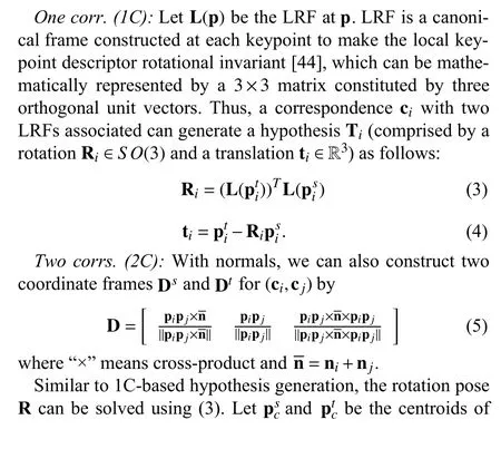
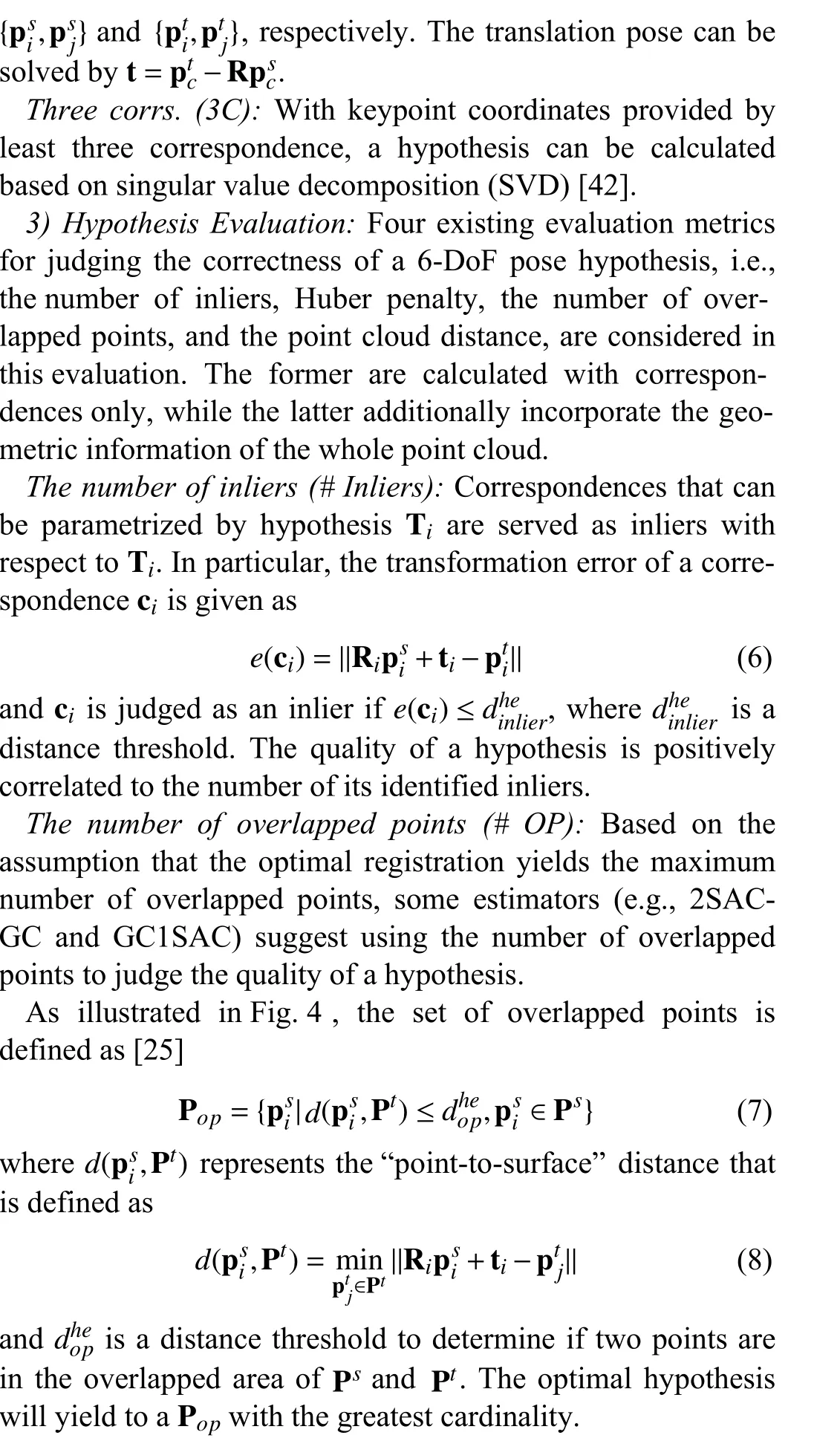
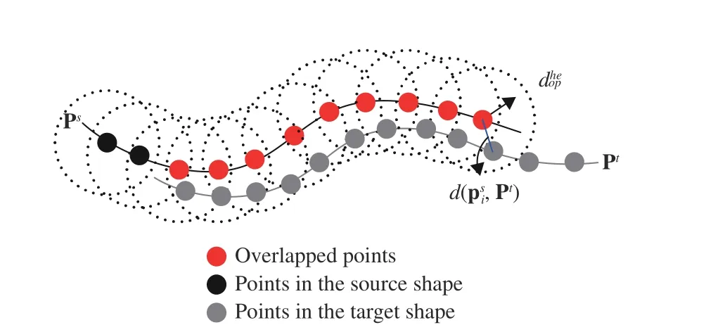
Fig. 4. Illustration of the set of overlapped points and “point-to-surface”distance ((7) and (8)).

Huber penalty (HP):Instead of classifying correspondences as inliers or outliers, HP scores a correspondence via

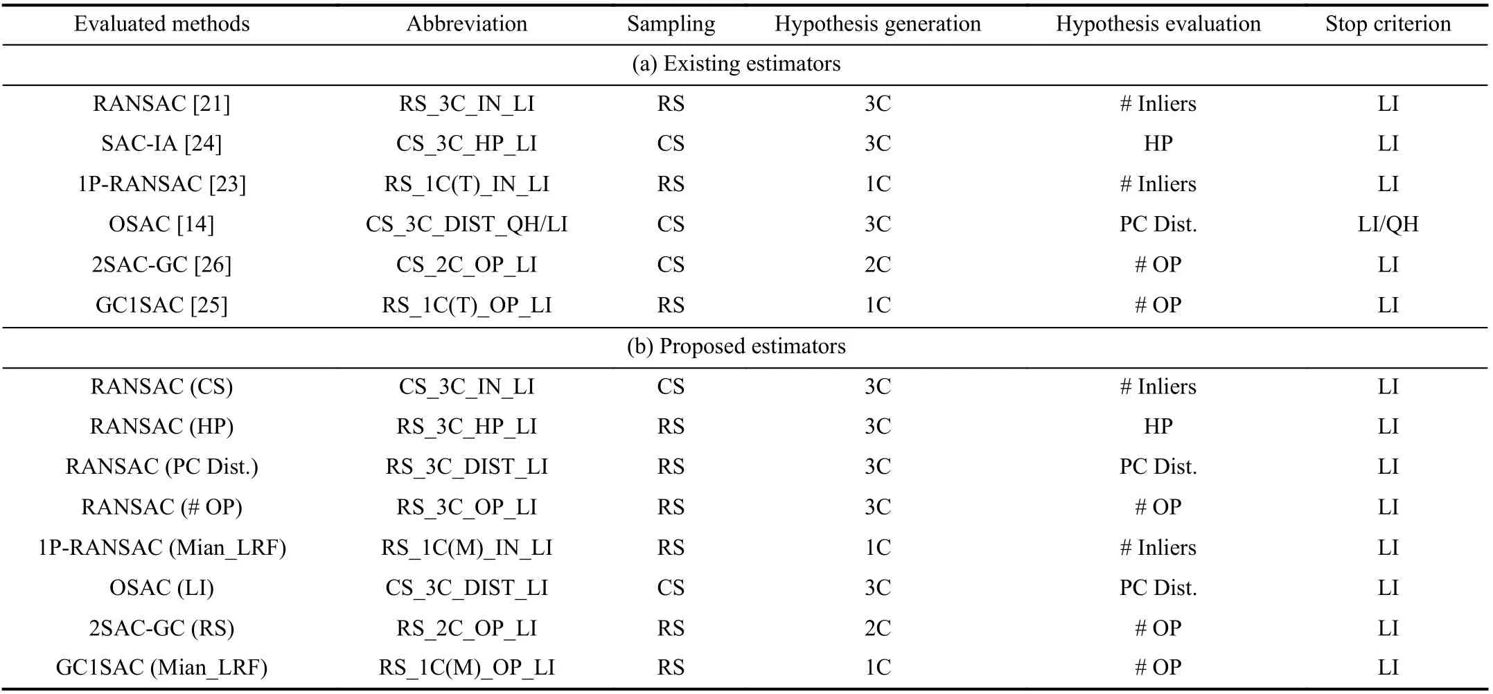
TABLE I A SUMMARy OF THE KEy STAGES OF CONSIDERED 6-DOF ESTIMATORS

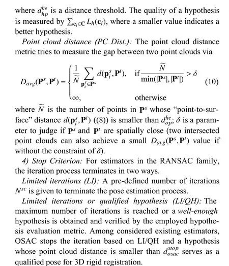
After describing existing methods in each key stage, we summarize the core technical components of six existing estimators considered in our evaluation in Table I(a). It also helps to highlight the common traits and differences of these estimators. To make the evaluated estimators easy to keep track of,we give a systematic name (the second column of Table I) for each evaluated method according to its computational procedure.

B. Proposed Estimators

Exploring the effects of each key stage on the overall pose estimation performance is important to explaining the comparative results, however, solely comparing existing estimators is not sufficient to achieve such a goal. For instance, evaluating RS_3C_IN_LI, CS_3C_HP_LI, RS_1C(T)_OP_LI, and CS_3C_DIST_QH/LI, we are still not able to fairly compare hypothesis evaluation metrics, because the differences of these estimators are not limited to the hypothesis evaluation stage.Therefore, we propose several variants of RANSAC, as shown in Table I(b), to particularly evaluate the performance of sampling strategies, hypothesis generation methods, hypothesis evaluation metrics, and stop criteria.

1) Sampling:CS_3C_IN_LI is proposed, as a competitor to RS_3C_IN_LI, to compare different 3-point sampling strategies; RS_2C_OP_LI is proposed to evaluate the performance of different 2-point sampling methods when compared with CS_2C_OP_LI. Note that 1-point sampling methods have a linear computational complexity and usually consider all correspondences as samples, neither using RS nor CS sampling methods. Therefore, we concentrate on evaluating 3-point and 2-point sampling methods.

2) Hypothesis Generation:1C-, 2C-, and 3C-based hypothesis generation methods rely on point coordinates, point coordinates + normals, and point coordinates + LRFs, respectively.In particular, the LRF cue is not as stable as normals and point coordinates [38], [44]. In addition, the quantitative effects of using LRFs with different repeatability behaviors remain unclear. Therefore, other than the LRFs employed by RS_1C(T)_IN_LI and RS_1C(T)_OP_LI (proven to exhibit good repeatability [44]), we also consider a far less repeatable LRF method, i.e., the one proposed by Mianet al. [45], and propose RS_1C(M)_IN_LI and RS_1C(M)_OP_LI.

3) Hypothesis Evaluation:We evaluate existing hypothesis evaluation metrics within the framework of RANSAC. In particular, we propose three RANSAC variants with different hypothesis evaluation metrics, i.e., RS_3C_HP_LI, RS_3C_DIST_LI, and RS_3C_OP_LI, and evaluate them paired with RS_3C_IN_LI to compare considered hypothesis evaluation metrics.

4) Stop Criterion:Most estimators stop iteration based on LI, except for CS_3C_DIST_QH/LI. Compared with LI,LI/QH employed by CS_3C_DIST_QH/LI could achieve a trade-off between accuracy and efficiency. To quantitatively examine such trade-offs, we propose CS_3C_DIST_LI as a competitor to CS_3C_DIST_QH/LI.

III. EVALUATION METHODOLOGy

This section presents the proposed evaluation methodology for considered 6-DoF pose estimators, including datasets,evaluation metrics, tested terms, and implementation details.

A. Datasets

Four publicly available datasets are considered, i.e., UWA 3D modeling (U3M) [46], Bologna Mesh Registration (BMR)[47], UWA 3D object recognition (U3OR) [45], [48], and Bologna Dataset5 (BoD5) [47]. Several sample views of shape pairs from these datasets are shown in Fig. 5.

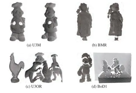
Fig. 5. Sample views of shape pairs from four experimental datasets.

The main properties of the four experimental datasets are summarized in Table II. Notably, U3OR and BoD5 are 3D object recognition datasets with available “SS-TS” settings.However, U3M and BMR are 3D registration datasets with no available “# SS” and “# TS” information. In particular, every shape pair in these two datasets can be a SS-TS pair if they have at least 10% overlap. Thus, we only give the number of qualified matching pairs for U3M and BMR in the table.These datasets have three peculiarities.i)Different application scenarios. 6-DoF pose estimation has been widely applied to 3D point cloud registration and 3D object recognition [4], [46], both of which are considered in our experimental datasets.ii)A variety of nuisances. These datasets provide a variety of nuisances for a comprehensive evaluation, e.g.,clutter, occlusion, self-occlusion, noise, and holes.iii)Different data modalities. Datasets acquired by a high-precision LiDAR sensor and a low-cost Kinect sensor are considered,resulting in point clouds with varying sparsities and qualities.Therefore, these datasets can generate initial correspondence sets with a variety ofinlier ratios,spatial distributions, andscales, which are three critical factors to a comprehensive evaluation of 6-DoF pose estimators. Fig. 6 visualizes several generated correspondence sets for four sample shape pairs from the experimental datasets.

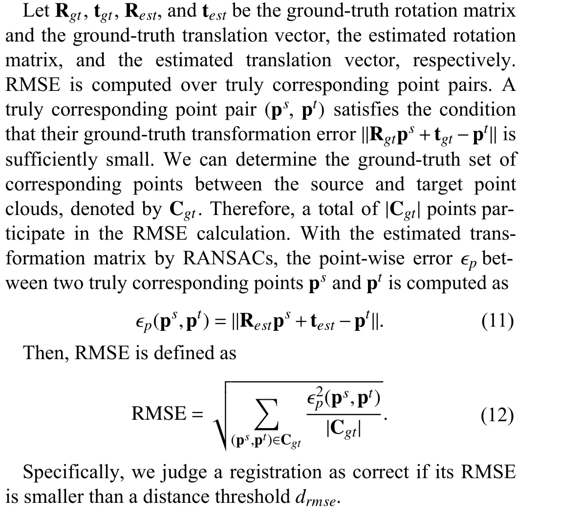
B. Metrics

For the assessment of 3D rigid registration accuracy, the root mean square error (RMSE) [14], [49], [50] criterion is employed.

C. Tested Terms

The quality of a 6-DoF pose estimator is determined from several critical aspects, e.g., 3D rigid registration accuracy,robustness to different experimental configurations, and computational efficiency.

1) Registration Accuracy on Different Datasets:The experimental datasets have different application contexts and various kinds of nuisances. Therefore, we first examine the registration accuracy performance of considered 6-DoF pose estimators on each experimental dataset. Because the accuracy requirement may vary with different applications, we vary the RMSE thresholddrmsefrom 1 pr to 10 pr with an interval of 1 pr. Here, the unit “pr” denotes the point cloud resolution, i.e.,the mean of the distances between each point and its nearest neighbor in the point cloud.

2) Registration Accuracy w.r.t. Different Configurations:In order to address some basic concerns for a 6-DoF pose estimator, we experiment with datasets in the following configurations. In particular, the following experiments are conducted on the U3M dataset, because it is the largest-scale dataset among experimental datasets and it contains high-quality point clouds that are suitable for injecting and assessing the effects of different levels of synthetic nuisances.

Gaussian noise:Noise are undesired points near a 3D sur-face [51]. We inject the target shape with different levels of Gaussian noise. Specifically, the standard deviation of Gaussian noise increase from 0.5 pr to 3.0 pr with a gap of 0.5 pr.The noise is injected from thex-,y-, andz-axis of each point.Fig. 7 (the second column) visualizes a point cloud with 1.5 pr Gaussian noise.

TABLE II ExPERIMENTAL DATASETS AND INHERITED PROPERTIES (SS: SOURCE SHAPE; TS: TARGET SHAPE)

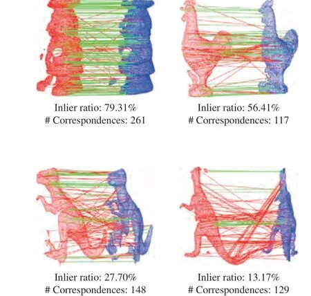
Fig. 6. Four sample correspondence sets with different inlier ratios, spatial distributions, and scales.

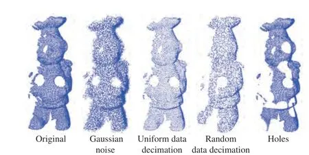
Fig. 7. Visualization of point clouds with different nuisances. From left to right: noise-free point cloud and point clouds with 1.5 pr Gaussian noise, 60%uniform data decimation, 60% random data decimation, and 14 holes, respectively.

Uniform data decimation:The variation of the distance from the sensor and the object/scene will result in point clouds with different densities. Therefore, we perform uniform downsampling on the target shape. In particular, approximately 80%, 60%, 40%, 30%, 20%, and 10% original points are retained after uniform down-sampling. Fig. 7 (the third column) shows a point cloud with 60% uniform data decimation.

Random data decimation:In addition to data decimation,the non-uniform distribution of points remains another challenging issue. However, it has been overlooked in most previous evaluations. Hence, we randomly reject points in the target shape, and keep approximately 80%, 60%, 40%, 30%,20%, and 10% original points, respectively. An exemplar view of a point cloud with 60% random data decimation is shown in Fig. 7 (the forth column).

Holes:Occlusion, self-occlusion, and materials with low reflectivity such as glasses, will cause holes in the acquired point clouds. We add 6, 10, 14, 18, 22, 26 holes to the target shape, respectively. Here, we synthesize a hole by first performing a k-nearest-neighbor (KNN) search for a point in the point cloud and then rejecting all neighboring points. The number of neighboring points is empirically set to 2%×|Pt|,where |Pt| represents the cardinality of point cloud Pt. Fig. 7(the fifth column) gives an exemplar view of a point cloud with 14 holes.

Varying scales of the input correspondence set:The correspondence set used for 6-DoF pose estimation is usually a subset of the initial correspondence set obtained by matching local keypoint descriptors [4], [14]. A popular way for obtaining such subset is to first rank correspondences based on some scoring rules [52], [53] and then selectNcorrtop-ranked ones.Here, we employ the Lowe’s ratio strategy [52] for correspondence ranking. Changing the value ofNcorrwill result in correspondence sets with different scales, inlier ratios, and spatial distributions. To test the effect of varying scales of the input correspondence set, we changeNcorrfrom 1 0%×|C| to 70%×|C|w ith a step of 1 0%×|C|.

Different detector-descriptor combinations:Because the correspondence set is obtained by matching local keypoint descriptors, the effect of selecting different detector-descriptor combinations should also be investigated. Specifically, two 3D keypoint detectors, i.e., Harris 3D (H3D) [54] and intrinsic shape signatures (ISS) [55], and three local geometric descriptors, i.e., signatures of histograms of orientations(SHOT) [56], spin image (SI) [57], and local feature statistics histograms (LFSH) [14], are selected due to their popularity[18], [19]. We use “C1 ～C6” to denote the combinations of“H3D+SHOT”, “H3D+SI”, “H3D+LFSH”, “ISS+SHOT”,“ISS+SI”, and “ISS+LFSH”, respectively. All these combinations are tested in our experiments.

3) Computational Efficiency:The average time costs of all tested pose estimators for registering a shape pair on the four experimental datasets will be recorded. This enables us to thoroughly compare the efficiency of each estimator because of the following reasons.

Fig. 8. Inlier information of four experimental datasets. (a) The overall information of the inlier ratio and the average number of inliers of experimental datasets; From (b) to (e): the statistical histograms of inlier ratios computed for four datasets.

First, the four datasets offer correspondence sets with different scales, spatial distributions, and inlier ratios, so the speed behavior of a pose estimator in different challenging conditions can be tested. Second, some tested estimators (e.g.,RS_1C(T)_OP_LI and CS_2C_OP_LI) also leverage the geometric information of the whole point cloud during hypothesis verification, the quantitative effect on the computational efficiency should be examined on datasets with different sparsities. In the experimental datasets, both sparse Kinect data and dense LiDAR data are included.

D. Implementation Details

Generation of the input correspondence set:By default, we use the H3D [54] keypoint detector and the SHOT [56]descriptor (i.e., the C1 combination mentioned in Section IIIC-2)) to detect keypoints on point clouds and describe local geometric features of keypoints, respectively. The initial correspondences are then generated by matching local geometric descriptors extracted from the source shape and the target shape based onL2distance.

With this setting, correspondence sets with different inlier ratios and inlier counts are generated for the experimental datasets as shown in Fig. 8(a). To further illustrate the characteristics of generated correspondence sets for each dataset, we give the statistical histograms of inlier ratios for the four datasets in Figs. 8(b)–8(e). In addition, the variety of inlier ratios and inlier counts is increased with different experimental configurations (Section III-C-2)) as shown in Fig. 9.

Remarkably, the goal of this evaluation is not to find the best detector-descriptor combination for 6-DoF pose estimation. We select H3D+SHOT because it can generate correspondence sets with varying inlier ratios, spatial distributions,and scales (as demonstrated in Figs. 7–9), which can enable a thorough evaluation.

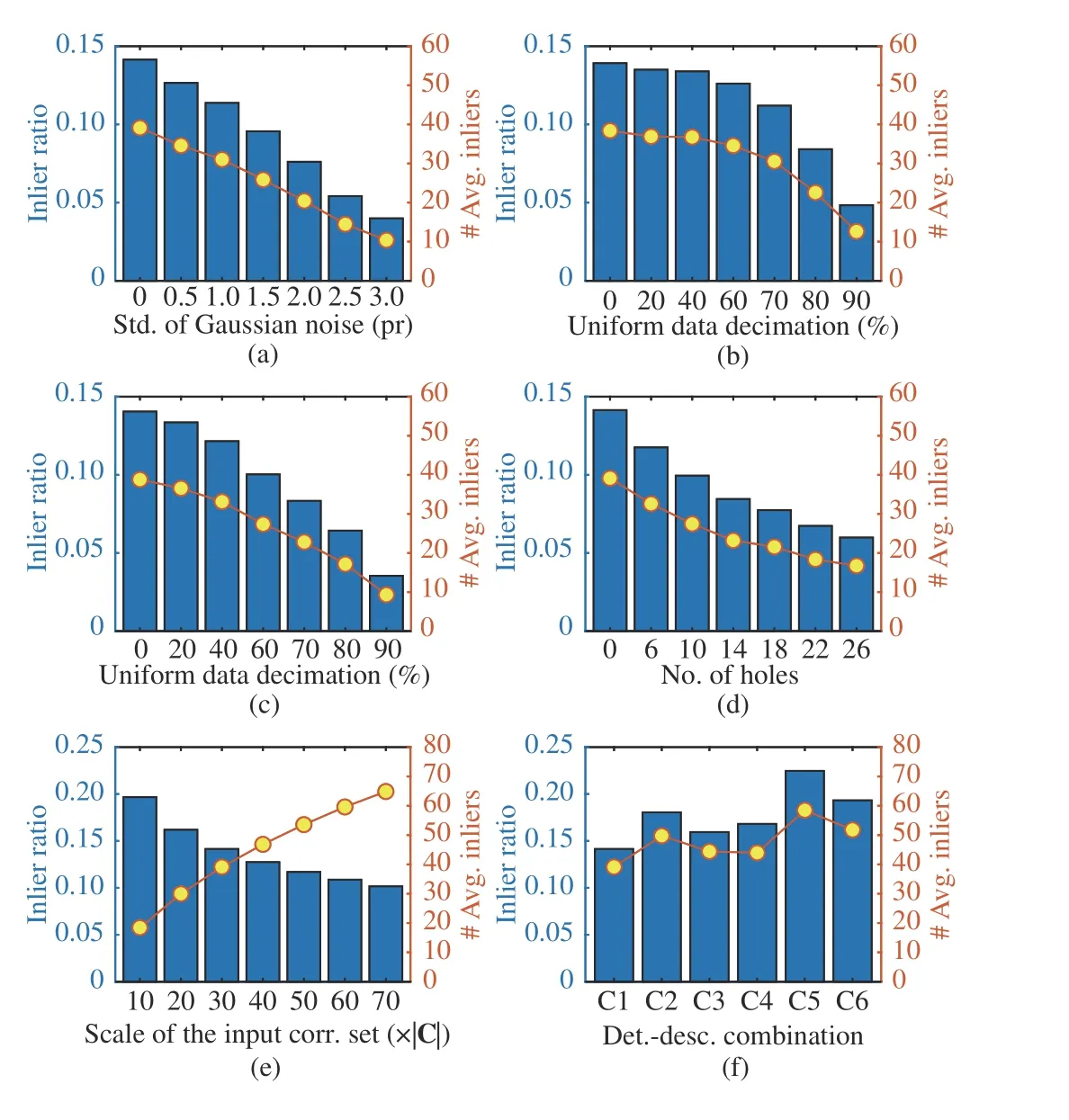
Fig. 9. Information in terms of the inlier ratio and the number of inliers of the input correspondence sets to evaluated estimators under different dataset configurations (Section III-C-2)). Bars indicate inlier ratio values, and dots indicate average inlier counts.

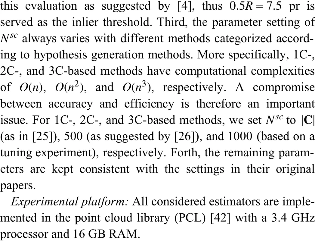
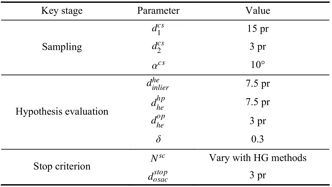
TABLE III PARAMETERS USED THROUGH THE EVALUATION (HG REPRESENTS HyPOTHESIS GENERATION)

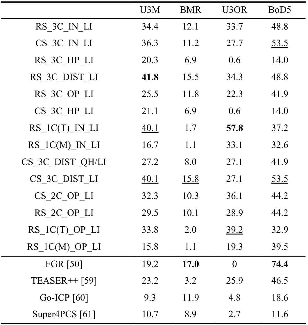
TABLE IV COMPARISONOF EVALUATED RANSAC METHODS WITH FOUR RECENT REGISTRATION APPROACHES IN TERMS OFREGISTRATION ACCURACy (%).HERE, drmse=5 PR;THEBESTANDTHE SECOND BEST ARE SHOWN IN BOLD AND UNDERLINE FACES, RESPECTIVELy)

IV. ExPERIMENTAL RESULTS

Based on the experimental settings in Section III, this section presents corresponding results with necessary explanations and discussions. To improve readability, in comparative result figures, solid and dotted lines represent random and conditional sampling methods, respectively; red, blue, and green lines represent 3C-, 2C- and 1C-based hypothesis generation methods, respectively; lines with *, +, ◦, and Δ markers represent different hypothesis evaluation metrics, i.e., the inlier (IN), Huber penalty (HP), point cloud distance (DIST),and the number of overlapped points (OP), respectively.

A. 3D Rigid Registration Performance on Different Datasets

For each estimator, we compute the percentage of its successfully registered point clouds on each dataset. For each dataset, we exclude shape pairs whose correspondence sets do not contain any inliers. The 3D rigid registration results of the evaluated 6-DoF pose estimators on four experimental datasets with respect to different RMSE thresholds are shown in Fig. 10. Several observations can be made from the figure.

Results on U3M:The main observations (Fig. 10(a)) are summarized as follows. First, CS_3C_DIST_LI and RS_3C_DIST_LI are two top-ranked estimators wheredrmseis smaller than 5 pr. RS_3C_DIST_LI outperforms other RANSAC variants with different hypothesis evaluation metrics, such as RS_3C_OP_LI and RS_3C_HP_LI, which indicates that “PC Dist.” can more accurately evaluate the quality of a hypothesis on this dataset. The superior performance of CS_3C_DIST_LI further verifies this conclusion. Second, by comparing RS_3C_IN_LI and CS_3C_IN_LI, we find that sampling correspondences that are distant from each other does not bring notable impacts. However, CS_2C_OP_LI behaves better than RS_2C_OP_LI which demonstrates the rationality of rejecting geometrically inconsistent samples.Therefore, the efficacy of conditional sampling depends on how the geometric constraints are defined. Third, Whendrmseis greater than 4 pr, CS_3C_HP_LI, RS_3C_HP_LI,RS_1C(M)_IN_LI, and RS_1C(M)_OP_LI are significantly inferior to other performers. Both CS_3C_HP_LI and RS_3C_HP_LI use the HP metric for hypothesis evaluation,which is shown to be far less effective than other metrics. As for RS_1C(T)_IN_LI and RS_1C(T)_OP_LI, they rely on LRFs for hypothesis generation and a clear performance deterioration occurs when less repeatable LRFs are used, i.e.,RS_1C(M)_IN_LI and RS_1C(M)_OP_LI. To better explain this result, we calculate the percentages of repeatable LRFs for experimental datasets when using TOLDI_LRF [58] (originally used in RS_1C(T)_OP_LI and RS_1C(T)_IN_LI) and Mian_LRF [48] and report the results in Fig. 11. Here, we follow [44] and define two associated LRFs of a correspondence as repeatable if their overall angular error is smaller than a threshold (10 degrees in this paper). The readers are referred to [44] for more details about the LRF angular error metric.Clearly, TOLDI_LRF generates more repeatable LRFs and 1C-based estimators with TOLDI_LRF deliver much better performance than those using the Mian_LRF.

Results on BMR:From Fig. 10(b), we are able to observe three phenomena. First, methods that leverage the whole point cloud for hypothesis evaluation exhibit superior performance,including CS_3C_DIST_LI, RS_3C_DIST_LI, and RS_3C_OP_LI. Compared with the results on the U3M dataset where methods using the “# Inliers” metric also show promising performance, results on this more challenging dataset (acquired via a Kinect sensor) suggest that metrics incorporating global point cloud information are more effective. Second, because both TOLDI_LRF and Mian_LRF show limited repeatability performance on this dataset (Fig. 11), all 1C-based methods suffer from limited performance. Third, we can find that RS_2C_OP_LI even surpasses CS_2C_OP_LI on this dataset.This is because of the noisy geometry information in this dataset, so the geometric constraints defined by CS_2C_OP_LI become unreliable. Therefore, good samples maybe missed when sampling correspondences for hypothesis generation.

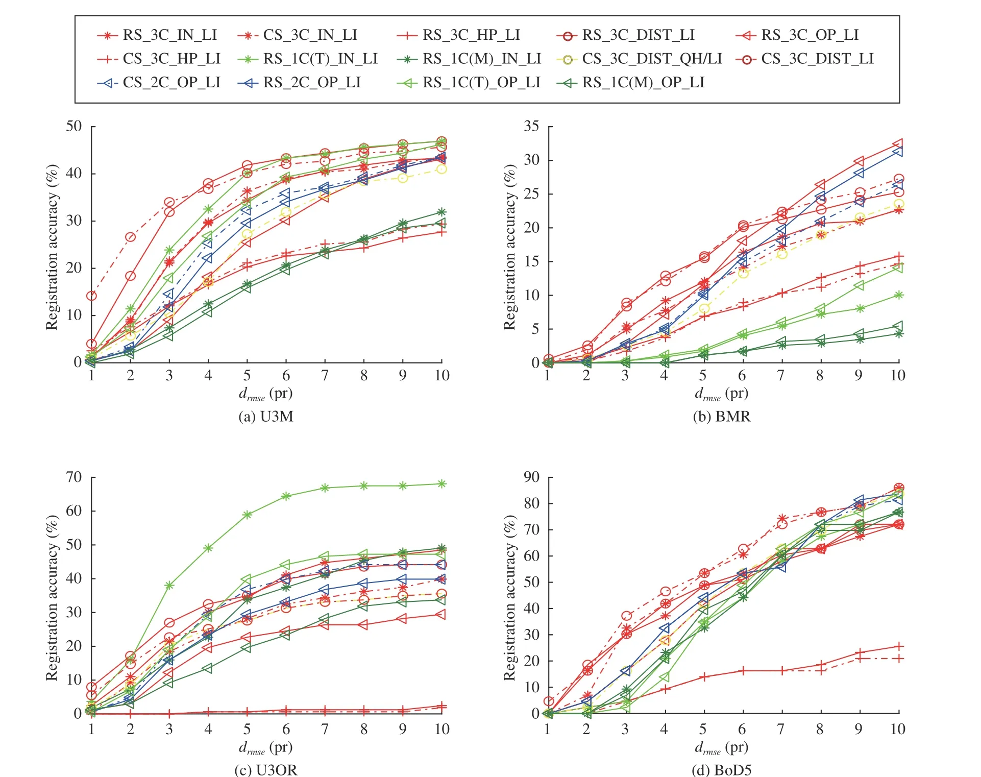
Fig. 10. 3D rigid registration accuracy performance of evaluated 6-DoF pose estimators on four experimental datasets with respect to different RMSE thresholds.

Results on U3OR:From Fig. 10(c), two salient observations can be made. First, RS_1C(T)_IN_LI outperforms others by a dramatic margin, including estimators with hypothesis evaluation metrics that leverage global point cloud information, e.g., RS_3C_DIST_LI and CS_3C_DIST_LI. However, these estimators generally achieve decent performance on point cloud registration datasets. Therefore, the effectiveness of hypothesis evaluation metrics including “# Inliers”, “#OP”, and “PC Dist.” tend to vary with application scenario and data modality changes. Second, methods with the “HP”metric, i.e., CS_3C_HP_LI and RS_3C_HP_LI, almost fail to register any shape pair on this dataset. Note that they also exhibit limited performance on U3M and BMR datasets. It arises from the fact that in a 3D object recognition scenario,the scene may contain many cluttered objects and false correspondences. Because “HP” is a continuous function (unlike other hypothesis evaluation metrics that assign binary labels to correspondences), the gap between the best scoring result and the remaining ones during iterations, may appear to be marginal for correspondences with heavy outliers. Furthermore, outliers will get significantly higher scores in the 3D object recognition scenario due to clutter, since they are in a more spatially sparse distribution than those in the point cloud registration scenario. As a result, CS_3C_HP_LI and RS_3C_HP_LI fail on this dataset.

Results on BoD5:In Fig. 10(c), one can see that except CS_3C_HP_LI and RS_3C_HP_LI, most methods achieve high registration accuracies and their performance gaps are relatively small. It is because the correspondence sets generated on this dataset contain the largest number of inliers and has the greatest inlier ratios among the four experimental datasets. Specifically, CS_3C_DIST_LI and CS_3C_IN_LI are the best two performers. It is interesting to note that CS_3C_IN_LI clearly outperforms RS_3C_IN_LI, indicating the positive impact of conditional sampling on this dataset.However, on the U3M and BMR datasets, RS_3C_IN_LI and CS_3C_IN_LI behave comparably; on the U3OR dataset,RS_3C_IN_LI surpasses CS_3C_IN_LI. A potential reason is that CS_3C_IN_LI tends to sample spatially dispersed correspondences as it assumes that such a sampling method is more likely to find inliers. Nonetheless, the spatial distributions of both inliers and outliers are observed to be unordered [20].Therefore, it results in inconsistent rankings for CS_3C_IN_LI and RS_3C_IN_LI on different datasets. Several points can be summarized based on the results in Fig. 10.First, the performance of methods using 1C-based hypothesis generation, e.g., RS_1C(T)_IN_LI and RS_1C(T)_OP_LI,heavily relies on the repeatability of their employed LRFs.Second, clear registration performance variation can be observed when using different hypothesis evaluation metrics.Among tested metrics, “HP” is inferior to others on all datasets. Third, the efficacy of conditional sampling depends on the stability of the employed geometric constraints forbadsample rejection. Forth, it is very challenging to consistently achieve good performance on datasets with different application scenarios and nuisances. The best estimator in crossdataset experiments is CS_3C_DIST_LI, which achieves decent performance on three of the experimental datasets, but results in a mediocre performance on the U3OR dataset.

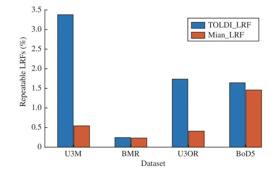
Fig. 11. Repeatability performance of two LRF methods (TOLDI_LRF [58]and Mian_LRF [48]) on four experimental datasets. TOLDI_LRF is originally used in RS_1C(T)_OP_LI and RS_1C(T)_IN_LI. Two associated LRFs of a correspondence are defined as repeatable if their overall angular error[44] is smaller than a threshold (10 degrees in this paper).

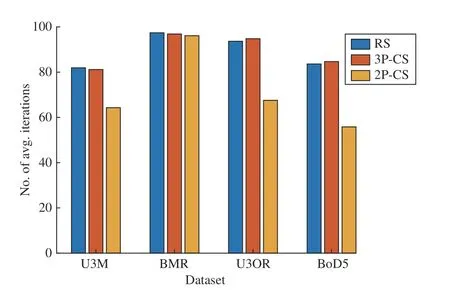
Fig. 12. Required average iterations of considered sampling methods, i.e.,random sampling (RS), 3-point conditional sampling (3P-CS) in CS_3C_HP_LI, and 2-point conditional sampling (2P-CS) in CS_2C_OP_LI,to achieve the first correct sample from correspondence sets on four datasets.

Fig. 10 also indicates that different sampling and hypothesis evaluation methods have obvious effects on final registration performance. Here, we conduct two experiments to compare the considered sampling and hypothesis evaluation methods. The former experiment tests the average required number of iterations of three sampling methods, i.e., random sampling (RS), 3-point conditional sampling (3P-CS) in CS_3C_HP_LI, and 2-point conditional sampling (2P-CS) in CS_2C_OP_LI, for achieving the first correct sample on four datasets. For the latter experiment, we first change the number of iterations in RANSAC such that various numbers of correct samples will be generated (less correct samplings indicating a more challenging problem for hypothesis evaluation);then RANSACs with four different hypothesis evaluation metrics, i.e., “# Inliers”, “HP”, “PC Dist.”, and “# OP”, are employed for registration. The results of these two experiments are reported in Figs. 12 and 13, respectively. Fig. 12 suggests 2P-CS can more reliably recognize good samples on U3M, U3OR, and BoD5 datasets. However, on the BMR dataset, due to noisy normals, 2P-CS just behaves like RS.These results indicate that more stable geometric constraints are desired to assist in effective conditional sampling.

For results in Fig. 13, we can make the following observations. First, we find that the overall method ranking outcome generally follows that of Fig. 10 on different datasets, i.e., the“PC Dist.” metric achieves the best overall performance on four datasets, even varying the number of RANSAC iterations from 100 to 1000. Second, increasing the number of iterations brings a more significant performance gain for “PC Dist.” and “# Inliers” on almost all datasets. Third, for “HP”on the U3M dataset, we find that its performance almost remains stable when giving more iterations. This can be explained that unconvincing hypothesis evaluation metrics,such as “HP”, are still not able to find correct samples when giving more iterations. Hence, the performance gain with more iterations is based on the reliability of the hypothesis evaluation metric.

Besides, to demonstrate that RANSAC methods can achieve state-of-the-art registration performance, we compare evaluated RANSAC methods with four recent registration methods,i.e., fast global registration (FGR) [50], TEASER++ [59], Go-ICP [60] and Super4PCS [61]. The results are reported in Table IV, which clearly indicate that RANSAC methods can still achieve outstanding performance even compared with recent state-of-the-art ones.This also suggests that RANSAC methods still worth evaluation.

B. 3D Rigid Registration Performance w.r.t Different Configurations

The robustness of each estimator is tested on datasets with different levels of Gaussian noise, uniform data decimation,random data decimation, holes, input correspondence sets with different scales, and different detector-descriptor combinations. Here, we fix the RMSE threshold as 5 pr. The number instead of the percentage of successful registrations is employed as the criterion in the following experiments,because the number of shape pairs withvalidcorrespondence sets (containing at least one inlier) may vary with different configurations. The results are shown in Fig. 14.

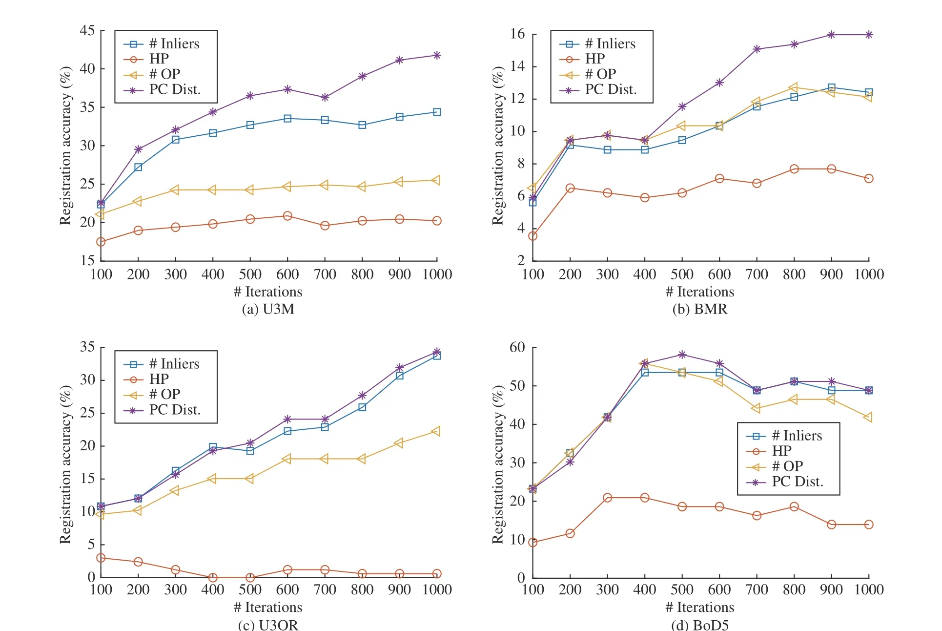
Fig. 13. Comparison of considered hypothesis evaluation metrics regarding registration accuracy (d rmse = 5 pr) when varying the number of iterations on four datasets.

Robustness to noise:Fig. 14(a) presents the results in the presence of Gaussian noise. First, CS_3C_DIST_LI is the best competitor under almost all levels of Gaussian noise. By contrast, CS_3C_DIST_QH/LI that terminates the iterative pose estimation process if the “PC Dist.” value of the registration is greater than a threshold, suffers from a significant performance drop. This indicates that a local minimum may be reached with the QH stop criterion. By contrast, if we use LI as the stop criterion, we may be in a lower local minimum or even a global minimum. Second, the performance of 1C-based methods, e.g., RS_1C(T)_IN_LI and CG1SAC, decreases dramatically as the Gaussian noise becomes severe. It is owing to the fact that the number of repeatable LRFs quickly decreases in the pretense of noise. Notably, it is still a challenging issue for existing LRF methods to achieve strong robustness to noise, as revealed by a recent evaluation of LRFs [44].

Robustness to uniform data decimation:Fig. 14(b) suggests that CS_3C_DIST_LI and RS_3C_DIST_LI are two topranked estimators under all levels of uniform data decimation.The performance of most estimators remains stable with less than 60% uniform data decimation and decreases more clearly when more points are decimated. In particular, the performance of some estimators, e.g., RS_1C(T)_OP_LI and RS_1C(M)_IN_LI, even improves with 20% uniform data decimation. It is because although uniform down-sampling removes points from the raw data, it can improve the uniformity of point distributions. When a small portion of points are removed, the overall geometry of point clouds can be preserved, while the remaining points are more uniformly distributed.

Robustness to random data decimation:As witnessed by Fig. 14(c), the performance of most estimators degrades even with a relatively small portion of points being randomly removed. It suggests that random data decimation is more challenging than uniform data decimation for tested estimators. RS_3C_DIST_LI and CS_3C_DIST_LI behave better than others with less than 80% data decimation; when more points are removed, RS_2C_OP_LI, CS_2C_OP_LI, and CS_3C_DIST_LI are the best three ones. It is noteworthy that methods with the “# OP” hypothesis evaluation metric, e.g.,RS_3C_OP_LI and CS_2C_OP_LI, are quite robust to random data decimation, their performance only degrades slightly even with 60% random data decimation. It indicates that the non-uniformity of point distributions has a faint impact on the hypothesis evaluation results by “# OP”.

Robustness to holes:Fig. 14(d) suggests that methods based on hypothesis evaluation metrics leveraging the whole point cloud information, e.g., RS_3C_DIST_LI, CS_3C_DIST_LI,CS_2C_OP_LI, RS_2C_OP_LI, generally achieve stronger robustness to holes than methods based on other metrics. The results demonstrate the effectiveness of considering global point cloud information when verifying hypotheses in the presence of holes. The reason is that the global shape geometry is more comprehensive and reliable when point clouds contain holes, compared with metrics (e.g., “HP” and “# OP”)using the information of correspondences only.

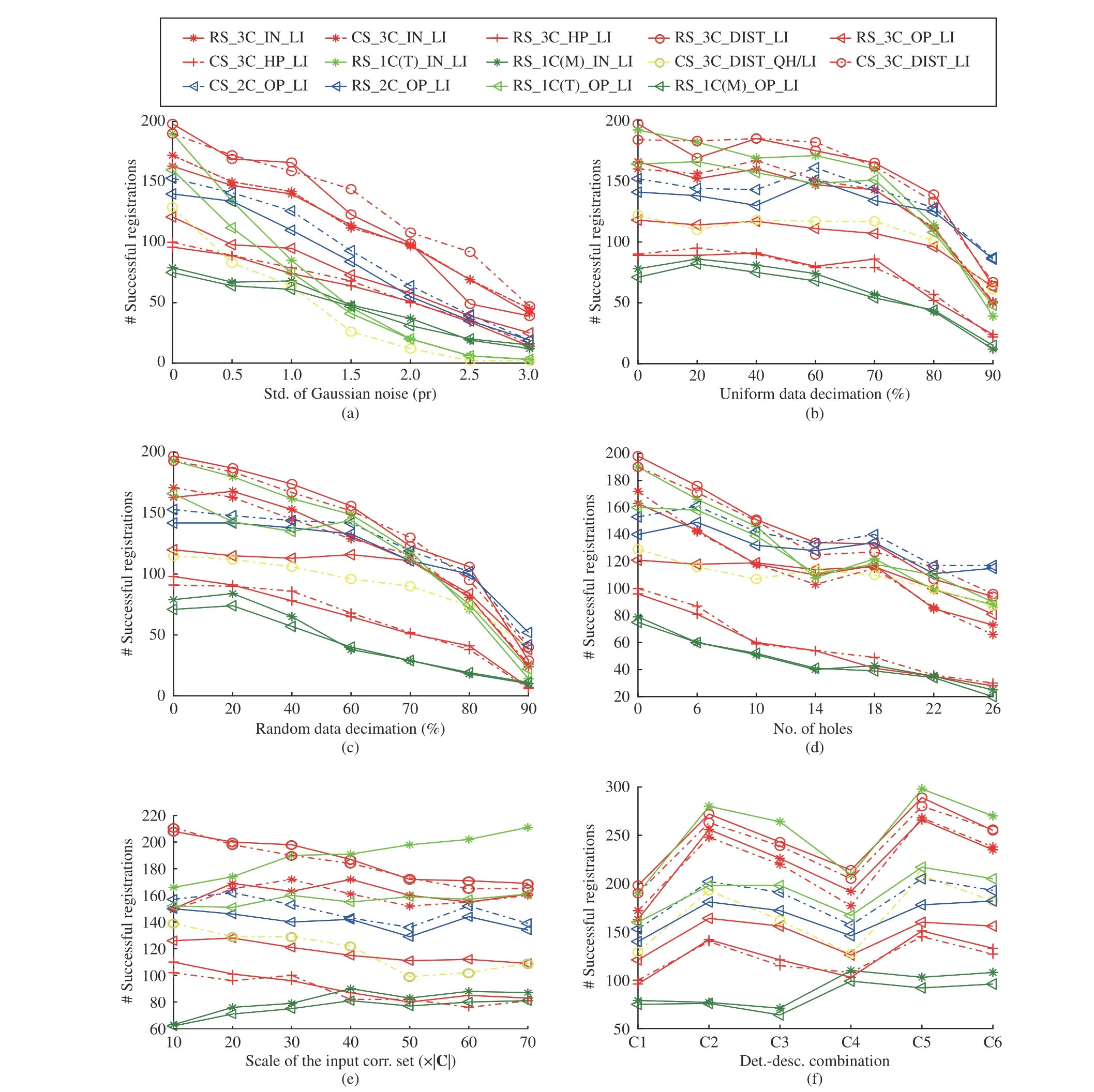
Fig. 14. 3D rigid registration accuracy performance of evaluated 6-DoF pose estimators with respect to different experimental configurations as presented in Section III-C-2).

Robustness to varying input scales:Fig. 14(e) shows that the performance of 1C-based methods climb as the scale of the input correspondence sets increases, whereas the performance of 2C-, and 3C-based methods generally decreases in this condition. Specifically, the phenomenon of performance deterioration is more salient to 3C-based methods. This is because the probability of finding good samples decreases for 2C- and 3C-based methods with a fixed number of iterations.For 1C-based methods, however, the probability of finding repeatable LRFs increases, so their performance improves when more correspondences are considered. One can see that RS_1C(T)_IN_LI outperforms the others by a clear margin when the scale of the input correspondence set equals 7 0×|C|.Theoretically, one correspondence with repeatable LRFs is sufficient to estimate an accurate 6-DoF pose for 1C-based methods.

Robustness to different det.-desc. combinations:As presented in Fig. 14(f), a clear performance variation can be found for most tested estimators when using different detector-descriptor combinations. However, the rankings of these estimators are relatively consistent. In particular,RS_1C(T)_IN_LI, RS_3C_DIST_LI, and CS_3C_DIST_LI consistently surpass the others with all tested detector-descriptor combinations. The performance gaps among evaluated estimators are less obvious when using C1 and C4 combinations. These observations show that the spatial distribution of correspondences is also a noteworthy factor for the 6-DoF pose estimation, which can result in significant impacts. For instance, C3 and C4 generate correspondence sets with similar inlier ratios and inlier counts (Fig. 9(f)), whereas the performance of estimators in these two detector-descriptor combination cases varies clearly. In general, nuisances including Gaussian noise, uniform data decimation, random data decimation, and holes are still very challenging for estimators in the RANSAC family. Specifically, RS_3C_DIST_LI,CS_3C_DIST_LI, and RS_1C(T)_IN_LI are three outstanding estimators among evaluated ones when tested on datasets with different challenging configurations.

Fig. 15. Average 6-DoF pose estimation time costs of evaluated estimators for registering a shape pair on four experimental datasets.

C. Computational Efficiency

The average 6-DoF pose estimation time costs of evaluated estimators for registering one shape pair on four experimental datasets are reported in Fig. 15.

Several observations can be made from the figure. First,estimators based on hypothesis metrics incorporating the global point cloud information are significantly more timeconsuming than others. As a result, even though 3C-based estimators have a computational complexity ofO(n3), many of them such as RS_3C_IN_LI and RS_3C_HP_LI are faster than some 1C- and 2C-based estimators (e.g., RS_1C(T)_OP_LI, CS_2C_OP_LI) by orders of magnitude. Therefore,for existing 6-DoF estimators in the RANSAC family, the most significant effects on the computational efficiency are brought by the hypothesis evaluation stage. Second, by taking the results of CS_2C_OP_LI and RS_2C_OP_LI into comparison, we find that rejecting samples based on effective geometric constraints can improve both registration accuracy and efficiency. However, the premise is that the defined geometric constraints are robust to common nuisances. Third, for CS_3C_DIST_QH/LI and CS_3C_DIST_LI, one can see that CS_3C_DIST_LI is more time-consuming but it surpasses CS_3C_DIST_QH/LI in terms of registration accuracy in all test conditions. This is mainly due to the fact that the employed hypothesis evaluation metric by CS_3C_DIST_QH/LI and CS_3C_DIST_LI fails to correctly judge the quality of hypotheses in many cases. Developing better hypothesis evaluation metrics remains one of the solutions to achieve a good trade-off between accuracy and efficiency. Forth, two 1C-based methods, i.e., RS_1C(T)_IN_LI and RS_1C(M)_IN_LI, are the two most efficient estimators. Notably,RS_1C(T)_IN_LI achieves outstanding registration accuracy performance in many tested conditions. Although they greatly rely on the repeatability of their employed LRF methods, they hold great potential to achieve both fast and accurate 3D rigid registration.

V. SUMMARy AND DISCUSSION

Based on the evaluation results, we first summarize the performance of tested methods and then present some interesting findings that may indicate new research directions in this research realm.

A. Performance Summary

The superior and inferior estimators in each tested case are shown in Table V. The following points can be summarized. i)On datasets with different application scenarios and data modalities, the performance of most estimators varies significantly. However, CS_3C_DIST_LI manages to be one of the best estimators on most datasets. Estimators using the “HP”hypothesis evaluation metric show poor performance, especially on 3D object recognition datasets. ii) On datasets with different configurations, CS_3C_DIST_LI and RS_3C_DIST_LI can resist the impact of a number of nuisances. By contrast,four estimators, i.e., RS_1C(M)_IN_LI, RS_1C(M)_OP_LI,CS_3C_HP_LI, RS_3C_HP_LI, are shown to be very sensitive to these challenging configurations. iii) RS_1C(T)_IN_LI and RS_1C(M)_IN_LI are the two most efficient estimators on all datasets. Notably, RS_1C(T)_IN_LI also achieves topranked performance in some tested conditions.

Therefore, it is still a very challenging issue for RANSACfashion 6-DoF pose estimators to achieve a balance in terms of accuracy, robustness, and efficiency.

B. Findings

This evaluation presents the following interesting findings that deserve future research attention.

1) Sampling:Because the distributions of both inliers and outliers are unordered [20], sampling correspondences based on their spatial locations cannot guarantee the quality of samples, as demonstrated by the results of RS_3C_IN_LI and CS_3C_IN_LI. Rejecting incompatible correspondences based on geometric constraints, as in CS_2C_OP_LI, is an effective way to improve the registration accuracy and efficiency. However, the efficacy is based on the stability of the employed geometric constraints. The ideal case is that all invalid samples are rejected using robust geometric constraints, which can be regarded as a pre-verification process for hypotheses to be generated, such that less iterations are required for hypothesis verification and the generated hypotheses are more consistent. Moreover, it is also interesting to mine other features such as colors and curvatures to guide conditional sampling [62].

2) Hypothesis Generation:For 3C-, 2C-, and 1C-based hypothesis generation ways, 1C-based methods possess an intriguing property, i.e., linear computational complexity.Although some 1C-based methods, e.g., RS_1C(T)_IN_LI,achieve superior registration accuracy performance in some experimental cases, their performance can be greatly limited by the repeatability performance of their employed LRFs.Unfortunately, existing LRF methods are still shown to be not repeatable in the presence of severe noise, clutter, and occlusion [38], [44]. This issue might be alleviated with the development of LRF techniques, however, it will be more interest-ing to investigate how to improve the stability of 1C-based methods even with less repeatable LRFs.

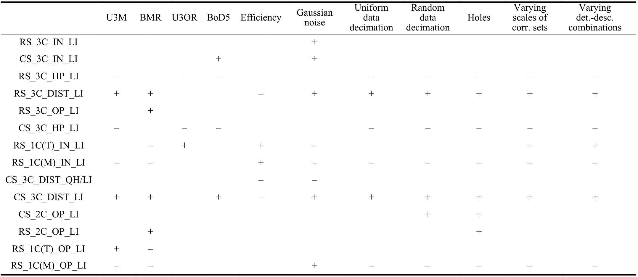
TABLE V SUPERIOR (+) AND INFERIOR (-) RANSAC-FASHION 6-DOF POSE ESTIMATORS SUMMARIzED BASED ON THE EVALUATION RESULTS IN SECTION IV

3) Hypothesis Evaluation:In the field of 3D rigid registration, the “PC Dist.” and “# OP” are recently proposed new metrics as compared with the traditional “# Inliers” metric.Although they are shown to be clearly better than the “#Inliers” metric in the original papers, our comprehensive evaluation reveals that the rankings of these three metrics vary with different data modalities, application contexts, and nuisances. Moreover, metrics incorporating global point cloud information are significantly more time-consuming. The “HP”metric is shown to be inferior to other metrics in all experimental conditions. Overall, before the definition of a good hypothesis evaluation metric, we should know how to define a good registration, i.e., is it a registration with sufficient consistent correspondences between point clouds, point clouds possessing the maximum number of overlapping points, or point clouds being spatially close enough? As indicated by our evaluation results, this remains a question to be answered with future research efforts. Moreover, other strategies to evaluate the registration results, such as visual evaluation and automatic recognition for registration evaluation, may be also integrated in the RANSAC pipeline and worth investigation.

4) Stop Criterion:“LI” is frequently used for existing RANSAC-fashion estimators as the stop criterion. Nevertheless, it usually needs lots of tuning experiments to determine the required number of iterations. “LI/QH” is a more flexible metric, however, it requires a convincing hypothesis evaluation metric as well, to discard redundant iterations and ensure registration accuracy.

VI. CONCLUSIONS

This paper has presented a thorough evaluation of several 6-DoF pose estimators in the RANSAC family for 3D rigid registration. In addition to the overall estimators, methods in each key stage have been comprehensively analyzed and evaluated,in order to on one hand explain the performance of evaluated estimators and on the other give hints for potential improvements on existing methods. Experiments were carried out on datasets with different application scenarios and configurations. This provides us with correspondence sets with a variety of inlier ratios, spatial distributions, and scales, thus enabling an in-depth evaluation. Based on experimental results, we give a summary of remarkable outcomes and valuable findings, in order to present practical instructions to realworld applications, and highlight current bottlenecks and potential solutions in this research realm.

In addition, this evaluation gives the following open issues.

1) RANSACs With Deep Learning:Deep learning techniques have achieved great successes in a number of computer vision tasks, including geometry-related ones such as point cloud registration [6], correspondence grouping [63],[64], and stereo matching [65]. For 2D image matching, some efforts have been made to improve the traditional RANSAC via deep learning, e.g., neural-guided RANSAC [66]. It will be therefore very interesting to see the performance of“RANSAC + deep learning” especially combined with point cloud geometric cues on 6-DoF pose estimation and 3D rigid registration, which may help overcome existing bottlenecks in this research field.

2) Push RANSACs to the Limit:Theoretically, RANSAC holds great potential for achieving fast and accurate 3D rigid registration, as long as correct samples are obtained in the early iteration stage and hypothesis evaluation metrics can efficiently dig out correct hypotheses. In other words, a “perfect” RANSAC can generate reasonable hypotheses without too many iterations and is able to quickly and correctly identify them. Thus, we believe that i) proposing guiding strategies to find correct samples within a few iterations, and ii)defining an efficient and reliable metric to evaluate the correctness of a registration without the ground-truth, are two critical directions for further improving RANSACs toward accurate, efficient, and robust 3D rigid registration.

ACKNOWLEDGMENTS

The authors would like to thank the Stanford 3D Scanning Repository, the University of Western Australia, and the University of Bologna for freely providing their datasets.