A new polar motion prediction method combined with the difference between polar motion series

Leyng Wng , Wei Mio , Fei Wu ,b

a Faculty of Geomatics, East China University of Technology, Nanchang 330013, China

b Key Laboratory of Mine Environmental Monitoring and Improving Around Poyang Lake, Ministry of Natural Resources, Nanchang 330013, China

Keywords:Earth rotation parameters Polar motion prediction LS+AR Differences between series Mean absolute error

ABSTRACT After the first Earth Orientation Parameters Prediction Comparison Campaign (1st EOP PCC), the traditional method using least-squares extrapolation and autoregressive(LS+AR)models was considered as one of the polar motion prediction methods with higher accuracy. The traditional method predicts individual polar motion series separately, which has a single input data and limited improvement in prediction accuracy. To address this problem, this paper proposes a new method for predicting polar motion by combining the difference between polar motion series.The X,Y,and Y-X series were predicted separately using LS +AR models. Then, the new forecast value of X series is obtained by combining the forecast value of Y series with that of Y-X series; the new forecast value of Y series is obtained by combining the forecast value of X series with that of Y-X series. The hindcast experimental comparison results from January 1, 2011 to April 4, 2021 show that the new method achieves a maximum improvement of 12.95% and 14.96% over the traditional method in the X and Y directions, respectively.The new method has obvious advantages compared with the differential method. This study tests the stability and superiority of the new method and provides a new idea for the research of polar motion prediction.

1. Introduction

The Earth rotation parameters (ERP) are necessary for the interconversion between the celestial reference frame and the earth reference frame.When the satellite navigation system enters the autonomous orbiting mode,or when the ground control system cannot upload the solved ERP, the system can only use the prediction of ERP [1]. Currently, space geodesic techniques such as Very Long Baseline Interferometry (VLBI), Global Navigation Satellite System (GNSS), Satellite Laser Ranging (SLR), Lunar Laser Ranging (LLR), and Doppler Orbitography and Radio Positioning Integrated by Satellites(DORIS)can be used to observe ERP.As the most important member of ERP, the prediction accuracy of polar motion(PM)has been the focus of satellite navigation orbiting and deep space exploration users. The polar motion is measured with high accuracy,but it is often necessary to upload the polar motion forecast values to the system in advance. Due to the complexity of the model for solving the polar motion in ground control centers[2],it is time-consuming and often delayed by hours or even days.Therefore, the development of new algorithms for polar motion forecasting is of great importance in solving this practical application problem.

In the study of polar motion forecasting, Zhu was the first to develop a least-squares harmonic model based on the periodic characteristics of the polar motion series and fitted the variation of the polar motion series[3].Chao analyzed the predictability of the polar motion by taking the trend,anniversary,and Chandler terms into account, performed least-squares extrapolation through the harmonic model, and proposed a forecast model for the floating period based on the time-varying nature of the polar motion period[4]. Kosek et al. regarded the fitting residual series of the leastsquares harmonic model as a stationary random series, then predicted it after the solution of the autoregressive model, and proposed the classic least-squares extrapolation and autoregressive(LS + AR) models [5,6]. After that, many scholars conducted improvement research based on the LS+AR models.In solving the LS model parameters, Sun et al. designed the weight array according to the distance from the predicted values [7]. Wu et al.combined the polar motion solution accuracy of International Earth Rotation Service (IERS) with that of International GNSS Service(IGS)to design the weight array[8].The prediction accuracy will be greatly affected when the LS model uses different input data lengths. Xu et al. experimentally derived a superior polar motion forecast accuracy for an input data length of 10 years[9].Based on the length of the input data for AR model, Wu et al. discussed empirically [10]. For the period of the polar motion series, Zhang et al. made a time-varying correction to the Chandler parameter,which effectively improved the forecast accuracy in the mediumlong term [11]. Sun et al. also used spectral analysis to probe the presence of weak inverse anniversary and semi-annual terms in the polar motion series[12].For the LS model,Wei et al.compared the effect of the presence or absence of the linear trend term on the forecast accuracy. They experimentally showed that the linear trend term appears to be particularly important for the mediumlong term forecast results [13]. Yao et al. observed a certain correlation between adjacent experiments and used the forecast error of the previous period to correct additional parameters for the forecast results of the next period, which effectively improved the short-term forecast accuracy [14]. Xu et al. combined the Kalman filter with the LS+AR models,effectively improving the short-term forecast accuracy [15]. Jia et al. improved the LS + AR models separately,one using Kalman filtering to modify the AR model and the other using minimum mean square error adaptive filtering to enhance the LS model. Both modification algorithms effectively improved the forecast accuracy of polar motion [16]. It is worth noting that the above studies are based on LS+AR models.They all forecast the polar motion of X series and Y series separately.There are relatively few studies that consider both polar motion series simultaneously. Song et al. solved the LS model parameters by putting the X series and Y series together [17]. Wang et al. developed a multiple autoregressive (MAR) model by composing the fitted X and Y residual series,and inputting them simultaneously to the MAR model to solve the model parameters [18]. Although the above two studies treated the X and Y series together, they still ended up in a single series forecasting approach.

The X-direction and Y-direction of the polar motion remain perpendicular in the two-dimensional plane. When geophysical excitation sources and other celestial bodies act simultaneously on the Earth rotation axis, the magnitude of the forces is recorded by astronomical means of observation in the form of X series and Y series. Since these internal and external forces act simultaneously on the Earth rotation axis, the major periods of the X series and Y series are the same.The Earth rotation axis makes an approximate elliptical motion with the Earth's body, and the X-direction and Ydirection are the coordinate direction decomposition of several ellipses.The X series and Y series are approximated as semi-ellipses when inscribed separately. On the one hand, when we try to form an ellipse out of these two semi-ellipses, the Y-X series describes this difference in information from an incomplete ellipse to a complete ellipse.On the other hand,the observation conditions of X series and Y series are the same,and the Y-X series may eliminate some common misinformation. At the same time, some useful high-frequency change terms may be weakened or enhanced.

In the first six-day forecasting method of phase 1, the researchers obtain a high short-medium term prediction accuracy in the excitation domain through the difference between ERP and EAM series in the same direction[19].This may be since the highfrequency excitation of the polar motion short time scale is mainly from the EAM,and the high-frequency term is effectively enhanced by the superposition of the difference series and the EAM series,thus obtaining a better forecast accuracy of 1-90 days. The prediction method provides a reference for this paper[19].In contrast,this paper focuses on the difference between X and Y series in different directions. With the help of this difference series of Y-X,the forecast value of the target series is obtained indirectly. Some practical high-frequency change terms may be diminished or enhanced with mathematical operations after combining the X, Y,and Y-X series.This new Y-X data,linked by mathematical relations,greatly enriches the form of polar motion input data. At the same time, the introduction of the new data (Y-X) corresponds to the addition of constraints on the acquisition of the target series in the forecast stage, which provides the possibility to obtain higher accuracy of the polar motion forecast.

The differential method [20-23] is similar to the new method.The difference is that the Y-X series or X-Y series introduced in this paper belong to the corresponding positions between the polar motion series for subtraction,which does not change the length of the input data. The differential method is a staggered subtraction within a single polar motion series,which will reduce the length of the input data.The differential method uses the internal difference information of a single polar motion series,which aims to enhance the smoothness of the individual series and thus better fit the AR model. Therefore, the new and differential methods are two different methods. The new method obtains the forecast value of the target series by combining the difference series with either series based on the difference information between the two series.This combination combines the forecast values of two AR models,which corresponds to the addition of constraints and outperforms the forecast accuracy obtained by the differential and traditional methods using a single AR model.

2. Model

2.1. LS extrapolation model

The mechanism of polar motion is very complex and mainly includes the long-term trend, Chandler oscillator, annual term,seasonal term, and high-frequency oscillator. The LS extrapolation model contains a constant term,a trend term,and a periodic term,and the model can be well fitted to extrapolate changes in the linear trend and periodic terms of the polar motion series [5,6]. The LS model is shown in formula (1).

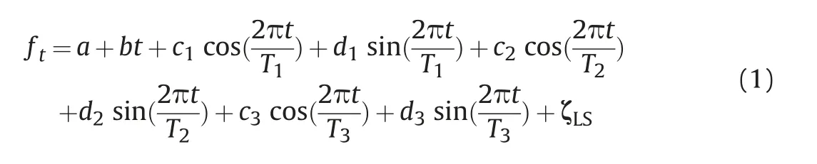
where ftrepresents the observation value of the polar motion at t,and t represents time series. a, b, c1, d1, c2, d2, c3, and d3are LS model parameters. ζLSrepresents the LS model fit residual. T1denotes the period value of the chandler term,with a value of 1.183a;T2defines the period value of the annual term, with a value of 1a;and T3denotes the period value of the semi-anniversary item,with a value of 0.5a, where 1a is 365.24 days [13].

All experiments in this paper use the Chandler,anniversary,and half-anniversary terms. After adding the 1/3- and 1/4-anniversary terms, and using the 2, 3, 4 and 5-period terms, the corresponding MAE figures can be viewed at the following link: https://efss.qloud.my/index.php/s/krxqm6zCT9sMnjL.

2.2. AR model

The AR model represents the relationship between the regular changes of random series and white noise [5,6,24]. The difference between the polar motion observations and the fitted values obtained by the LS model is the fitted residual series.The above fitted residual series is input into the AR model.The AR model is shown in formula (2).

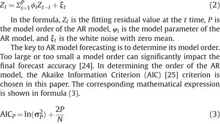
In the formula,σ2Pis the variance of the fitted residual series,N is the length of the input data,P represents the model order,and the value of P is much smaller than the value of N.

If S is the upper limit of the search interval,then P searches from 1 to S,and the value of P changes with the value of AICP.When the value of AICPreaches the minimum, the corresponding P value is the optimal order.Before using the AIC criterion to determine the P value, the search interval set in each experiment of this paper is from 1 to 300.

2.3. Solving model parameters

When solving the model parameters, the least square method has high computational accuracy and unbiased estimation due to its computational simplicity [24]. Therefore, this paper uses the least square method to calculate the model parameters of the LS +AR models, as shown in formula (4):

In the formula, B represents the coefficient matrix, and X represents the model parameter. When solving the LS extrapolation model parameters, L denotes the matrix consisting of the polar motion observation series;when solving the AR model parameters,L represents the matrix consisting of the fitted residual series.

3. Method

3.1. Traditional method

The Institute of Geodesy and Geophysics of the Vienna University of Technology organized the 1st EOP PCC between 2005 and 2008. At the end of this forecasting competition, the LS + AR models were considered as one of the polar motion predicting methods with high accuracy [26]. The traditional method is based on LS+AR models,where the first one of the series of polar motion is input into the LS model. Then the fitted values of the known phase and the forecast values of the extrapolated phase are obtained. The fitted values obtained by the LS model are subtracted from the input data of the known phase to acquire the fitted residual series of the known phase.The fitted residual series are then input to the AR model,and the forecast values of the fitted residual series will be obtained after processing by the AR model.Finally,the extrapolated forecasts obtained from the LS model and the fitted residual forecasts obtained from the AR model are superimposed to acquire the final estimates.The forecasts of the traditional method are denoted as XAi,YAi,where A represents the traditional method.A concise flow chart of the above steps is shown in Fig.1.

3.2. The new method

Based on the combined LS+AR models,the traditional method forecasts the X and Y series.On the basis of the traditional method,this paper adds a forecast experiment using Y-X series or X-Y series,thus constructing a new polar motion forecast relationship by introducing Y-X series. A concise flow chart is given below, as shown in Fig. 2.

Comparing Figs.1 and 2, it can be seen that Fig. 2 adds the experiments of Y-X series and constructs a new forecast relationship than Fig.1, and the rest of the steps are the same. The operation position of subtraction between polar motion series is before the LS model. A simple formula derivation and repeated experimental tests were conducted for the position of subtraction between series,and the following two conclusions were obtained. The choice of either Yi-Xiseries or Xi-Yiseries does not change the final forecast results.The final polar motion forecast results are obtained by performing the subtraction operation at the original series position. The fitted series position and the fitted residual series position are the same. Therefore, the operations of subtraction between series are chosen to be performed at the original series position of the polar motion for simplicity,and the forecast value of the Y-X series is noted as ΔCi ,where C represents the new method.

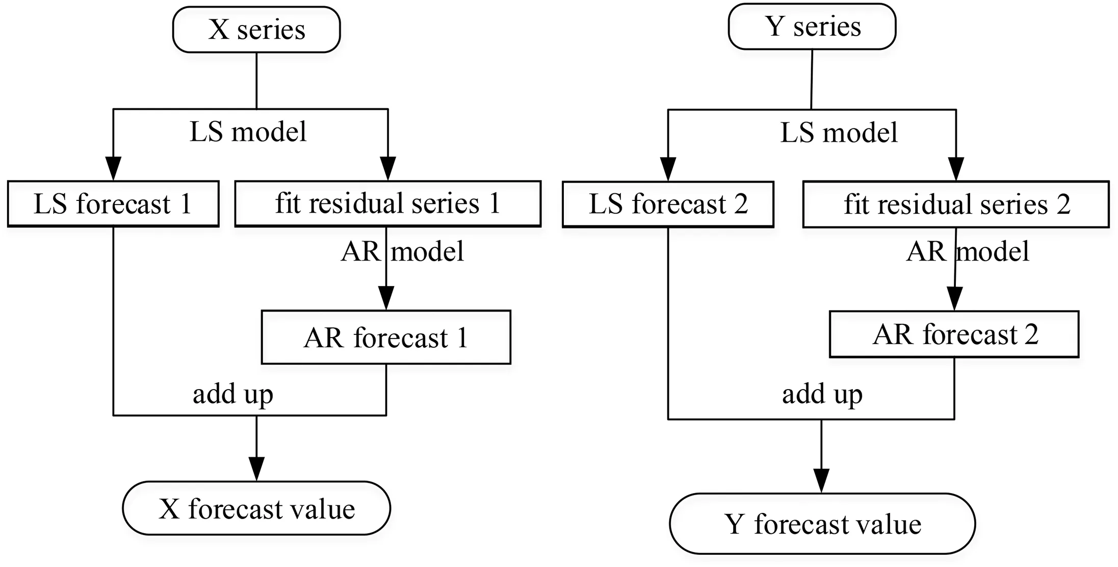
Fig.1. Prediction flowchart of the traditional method.

Fig. 2. Prediction flowchart of the new method.

It should be noted that the fitted and extrapolated forecasts of the X, Y and Y-X series will be obtained after the LS model processing. The fitted and extrapolated forecasts of the above three series still maintain Yi-Xiand （Y-X）iequivalence. On the one hand, at moment t, any time series is entered into the LS model,then the extrapolated forecast values have no relationship with the values at the last moment. On the other hand, the results of extensive and repeated tests show that the magnitude of the difference between the fitted and extrapolated forecasts of the LS model is smaller than that of 2×10-14.In other words,after the LS model processing, there is no change in the relationship between Yi-Xiand （Y-X）iequivalence. The above description can be verified by the attachment in the following link:https://efss.qloud.my/index.php/s/niRbew5eGYiyEms. All the changes in the results occur in the AR model, which changes the relationship between Yi-Xiand （Y-X）iequivalence. On the one hand, each forecast value of the AR model computed at time t requires the forecast value computed at the previous time,so that there is a dependency relationship.On the other hand,the fitted residual matrices of Yi-Xiand （Y-X）iare different, so the results obtained after the AIC criterion are also different, and the order of the AR model has a greater impact on the forecast accuracy.

As mentioned earlier,the forecast values of X series,Y series and Y-X series are XAi, YAiand ΔCi. Then after the adjustment of the AR model, a new relationship exists between XAi,YAiand ΔCi.The new forecast value of X series and Y series can be obtained according to the following formula (5).

3.3. Prediction error estimates

In order to verify the prediction effect obtained by the polar motion prediction algorithm, absolute error (AE), mean absolute error (MAE) and prediction accuracy improvement percentage(PAIP) are selected as the standards for prediction accuracy evaluation [16,24]. As shown in formulas (6), (7), and (8):

4. Experiment

4.1. Data selection

The experimental data are selected from the EOP 14C04 series published on the official website of the International Earth Rotation Reference Service (IERS). The EOP 14C04 series contains information on the polar motion,LOD,UT1-UTC,axial precession,nutation,and variance of the above series, with a sampling interval of one day.The X series and Y series from January 1,1996 to April 4,2021 are selected as experimental data. Among them, ten years (3652 days)and 15 years(5479 days)are chosen as the input data length for each experiment, respectively. Then, in testing the statistical forecast accuracy of the forecast algorithm, the forecast interval is from January 1, 2011 to April 4, 2021, i.e., the start of the first forecasting experiment is January 1, 2011, and the end of the last forecasting experiment is April 4, 2021. The forecast experiments were updated at an interval of one day, and the forecast experiments were repeated 3383 times on a sliding scale, with a forecast horizon of 1-365 days for each experiment.

4.2. Scheme design

In existing studies, the traditional method obtains better forecast accuracy when the input data length is ten years [9]. In this paper, it is found experimentally that this conclusion becomes a relative problem when a longer forecast interval is chosen to test the forecast method, and the magnitude of the effect of different input data lengths on the forecast accuracy of the traditional and new methods is explored separately. The differential method has been verified in papers[21-23]that the forecast accuracy obtained by making the difference at the fitted residual series position is better than that at the original series position.Therefore,first-order difference and second-order difference experiments with input data lengths ranging from 2 to 8 years are conducted at the fitted residual locations. Finally, the optimal forecast results of the differential method are selected for the comparison.

The above methods were designed into six experimental schemes, as shown in Table 1.

4.3. Results and analysis

After choosing the forecast interval from January 1, 2011 to April 4, 2021 and implementing the schemes, the MAE and PAIP values of the new and traditional methods can be calculated based on the forecast accuracy assessment formula in Section 3.3.Tables 2 and 3 list the MAE values of each forecasting method and the percentage improvement PAIP over the traditional method.Fig. 3 depicts the difference between the new and traditional methods under the same forecast conditions. In order to more clearly illustrate the advantages of the new method, Fig. 4 further shows the percentage improvement of the new method over the traditional method.

For the differential method, the first-order differencing gives better results in X-direction when the input data length is five years, and the second-order differencing gives better results when the input data length is six years. In Y-direction, the results obtained by first-order differencing are better when the input data length is three years, and the results obtained by second-order differencing are better when the input data length is six years. Since the forecast accuracy of the differential method is lower than that of the new method, their optimal forecast results are given in the last two columns of Tables 2 and 3, and the PAIP of the new method over the differential method is not calculated.

Tables 2 and 3 and Fig.3 depict the mean absolute error(MAE)of the new and traditional methods through different forms. The magnitude of the MAE value best reflects the forecasting capability of the forecasting method[26].Tables 2 and 3 show the MAE values in X-direction and Y-direction, which respectively correspond to the left panel and right panel of Fig. 3. By comparing the MAE values of the new, traditional and differential methods, it can beseen that the new method has different degrees of improvement over the traditional method and has a greater advantage over the differential method.

Table 1 Experimental schemes.

As can be seen from Table 2,the new method outperformed the traditional method in X-direction from days 2-365,except for day 1, which was slightly inferior to the traditional method, and this advantage was more obvious after 60 days.This may be due to the fact that the new method obtains the forecast values of X series by combining Y-X series and Y series, and the process involves a subtractive operation.The high-frequency term may be attenuated,while the high-frequency term mainly affects the forecast accuracy in the medium-long term.As seen from the left panel of Fig.4,the forecast accuracy of the new method shows an increasing trend,with the maximum percentage improvement reaching about 13%.The proposed new method effectively improves the forecast accuracy in the medium-long term for X-direction.

A comparison of the MAE values in Table 3 shows that the new method improves mainly from 1 to 150 days in Y-direction,with a maximum percentage improvement of about 15%.Then,combined with the right panel in Fig.4,it can be obtained that the PAIP of the new method over the traditional method reaches its maximum at around 90 days.The new method contributes to the short-medium term forecast accuracy in Y-direction,probably because the forecast values in Y-direction are obtained by summing the Y-X series and the X series.The operation of addition enhances the high-frequency term,which leads to a decrease in the accuracy of the medium-long term forecasts after 150 days. However, the high-frequency term retains more information, which will contribute to the short-term forecast accuracy.

Fig.3 shows that the forecast accuracy obtained using the input data length of 15 years is better than that of ten years in both directions. On the one hand, this may be the result of choosing a longer forecast interval.On the other hand,adding more input data to the model will help obtain a better forecast accuracy. The research suggests that a 10-year input data length yields better forecast accuracy [9], which is not a problem when tested on shorter forecast intervals. This issue becomes a relative problem when tested on longer forecast intervals.A new algorithm for polar motion forecasting is proposed,and a longer forecast interval needs to be chosen to test it.It is worth noting that the forecast interval of this paper is from January 1,2011 to April 4,2021,and the stability and applicability of the new method are well tested in this nearly 10-year forecast interval.

Comparing the forecast accuracy of the new method and the differential method in Tables 2 and 3, it is clear that the new method outperforms the differential method in terms of overall forecast accuracy. The results of established studies [20-23] show that the differential method only has a higher forecast accuracy in the short term. Tables 2 and 3 give the optimal forecasting results for first-and second-order differencing.However,the new method still has some advantages over the differential method in the short term. Therefore, although the new method is similar to the differential method, the new method has obvious advantages over the differential method.

After averaging all experiments, the forecast accuracy and its improvement percentage can only reflect the overall forecast level and stability of each method, but not the specific detailed characteristics. To address this issue, the forecast absolute error (AE)matrix is inscribed in Fig. 5. AE describes the difference of the forecast value relative to the observed value(EOP 14C04 series)for each forecast experiment.

Comparing the left and right panels of Fig.5,it can be seen that scheme 4 of the new method has advantages over the traditional method for 60-365 days in X-direction and significant advantages over the traditional method for the first 150 days in Y-direction.These advantages are mainly reflected in the forecast results from the 732nd experiment to the 2193rd experiment. Since the polar motion series are strongly periodic and most of the features of the historical series can be reproduced in the future,the new method is effective and feasible for upgrading the forecast accuracy of polar motion.To better demonstrate the advantages of the new method,the 732nd and 1462nd experiments were selected to compare the forecast values of the new method,the traditional method,and the observations from the EOP 14C04 series (Fig. 6).

Table 2 MAE and PAIP of the polar motion in X-direction.

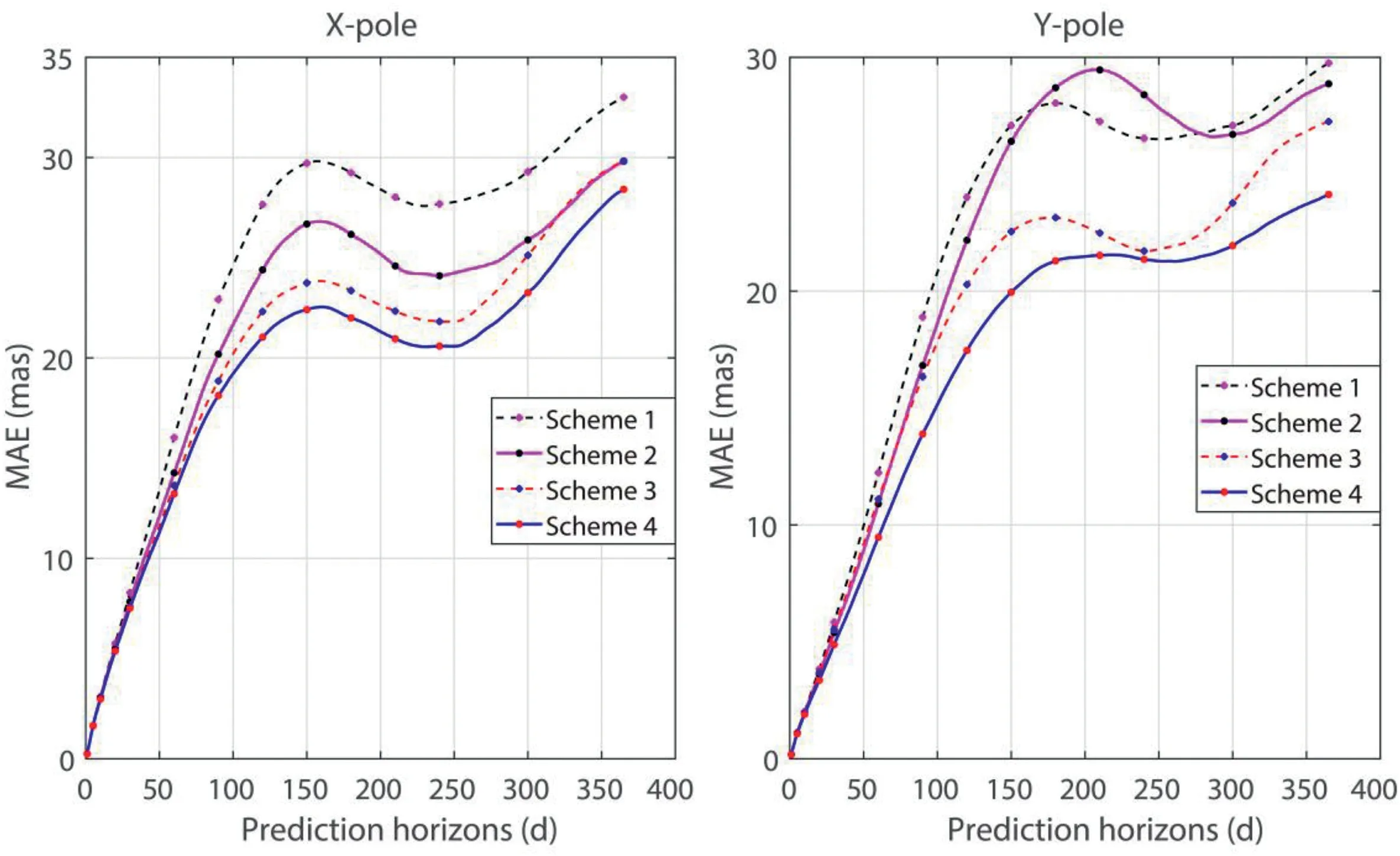
Fig. 3. Comparison of the forecast accuracy between the traditional and new methods.

As can be seen from Fig.6,the forecast values of the new method maintain the same trend as those of the traditional method,but the forecast values of the new method are closer to the observed values than those of the traditional method,which again indicates that the new method is practical and effective for polar motion forecasting.

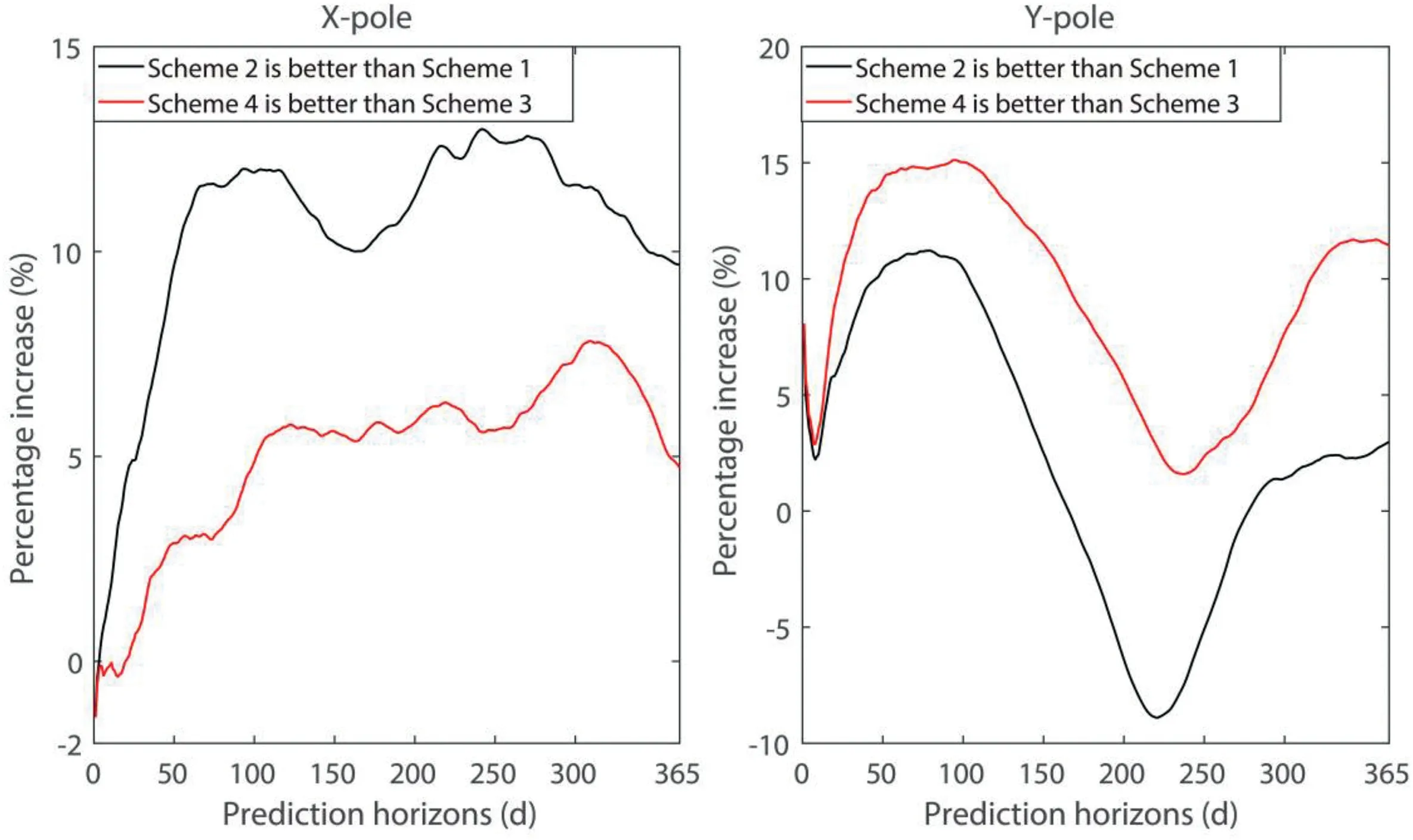
Fig. 4. PAIP of the new method over the traditional method.

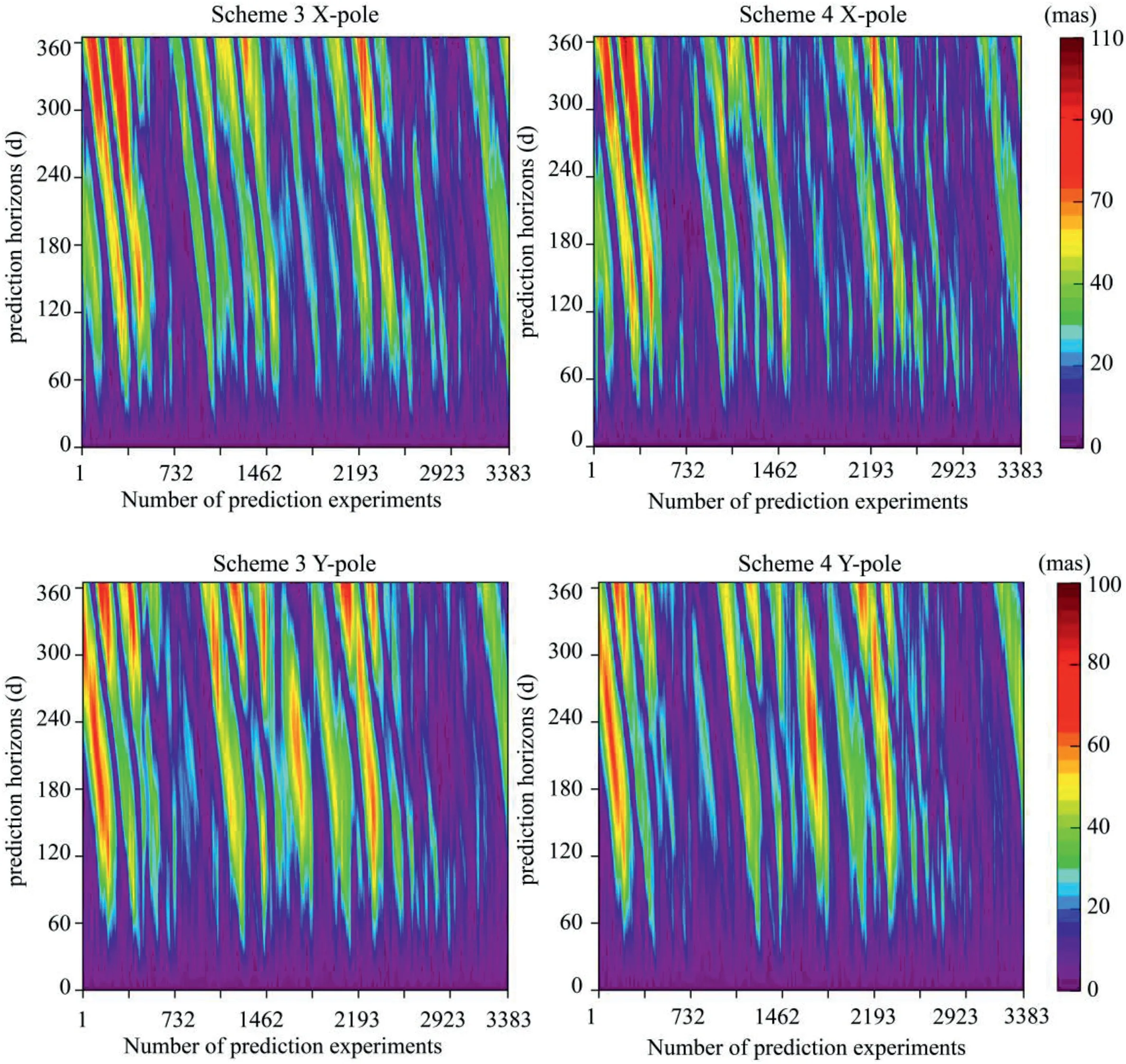
Fig. 5. The difference between the forecast values of the new method and the traditional method compared to the EOP 14C04 observation series. X-pole is the upper part, and Ypole is the lower part.The traditional method is unified on the left,and the new method is unified on the right.The numbers in the horizontal direction represent the location of the experiments,which can be converted to a specific date.The forecast experiments were updated every 1 day,and a total of 3383 experiments were conducted.The numbers in the vertical direction are the values on the prediction horizons,which is from 1 to 365 for each experiment. On the far right is the color reference standard,corresponding to formula(6), where the units have been converted to mas.

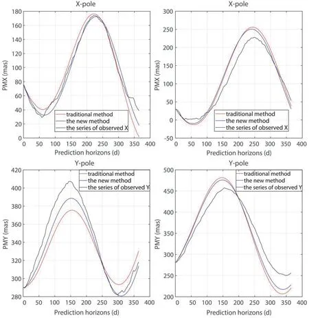
Fig.6. Comparison results of the forecast values of the traditional method,the new method and the observed values(EOP 14C04 series).The solid red line is the forecast value of the traditional method; the solid blue line is the forecast value of the new method; the solid black line is the observed value. In X-direction(upper part)and Y-direction(lower part),only the comparative results of the 732nd and 1462nd experiments are shown.The number on the horizontal axis indicates the prediction horizons size for each experiment;the number on the vertical axis indicates the value of the polar motion, and the units have been converted from as to mas.

5. Conclusion

To address the problem of a single form of input data for polar motion forecasting,this paper introduces a new dataset(Y-X series of polar motion), thus giving the forecasting method. Under the same forecast interval conditions, it can be seen after 3383 experimental tests that the new method has different degrees of improvement over the traditional method and has obvious advantages over the differential method. In summary, the following four works have been done in this paper.

(1) The difference series between the polar motion series is proposed for the first time.The new data and its forecasting method enrich the study of polar motion forecasting methods and have some reference value for future polar motion forecasting research.

(2) The effects of different input data lengths on the forecast accuracy of the new and traditional methods were investigated. Increasing the input data length can effectively improve the forecast accuracy of the new and traditional methods.

(3) The new method has a better improvement after 60 days in X-direction and higher forecast accuracy in the first 150 days in Y-direction.

(4) The new method and the differential method are distinguished and compared. The new method has obvious advantages over the differential method.

This paper uses fixed period values, and the next step of considering time-varying period values will further improve the forecast accuracy of the new method. Based on the combination idea proposed in this paper, a higher prediction accuracy is expected if some better models or methods are replaced to predict the Y-X series.

Author contributions

Leyang Wang:Conceptualization, Methodology, Supervision,Formal analysis, Investigation, Funding acquisition.Wei Miao:Conceptualization, Methodology, Software, Writing Original Draft,Writing-Review & Editing.Fei Wu:Resources, Suggestions.

Conflicts of interest

The authors declare that there is no conflicts of interest.

Acknowledgements

The authors are grateful to the anonymous reviewer for the comprehensive and insightful comments,which have improved the result presentation. We are also very grateful to the International Earth Rotation and Reference System Service (IERS) for the polar motion data. The work is funded by the National Natural Science Foundation of China(Nos.42174011 and 41874001),Jiangxi Province Graduate Student Innovation Fund (No. YC2021-S614), Jiangxi Provincial Natural Science Foundation(No.20202BABL212015),the East China University of Technology Ph.D. Project (No. DNBK2019181),and the Key Laboratory for Digital Land and Resources of Jiangxi Province, East China University of Technology(No.DLLJ202109).