Insights into spatio-temporal slow slip events offshore the Boso Peninsula in central Japan during 2011-2019 using GPS data

Meng Li , Li Yn ,c,*, Zhongshn Jing , Genru Xio

a Faculty of Geomatics, East China University of Technology, Nanchang, Jiangxi 330013, China

b Faculty of Geosciences and Environmental Engineering, Southwest Jiaotong University, Chengdu 611756, China

c Engineering Research Center for Seismic Disaster Prevention and Engineering Geological Disaster Detection of Jiangxi Province, East China University of Technology (Earthquake Administration of Jiangxi Province), Nanchang 330013, China

Keywords:Slow slip events (SSEs)GPS PCAIM Spatio-temporal evolution Boso peninsula

ABSTRACT Using Global Positioning System(GPS)coordinate time series,we detect three transient slow slip events(SSEs) offshore the Boso Peninsula in central Japan during 2011-2019. To extract the tiny SSE signals obscured by the significant post-seismic deformation after the 2011 MW9.0 Tohoku earthquake,we develop a new GPS coordinate time series processing software to obtain these SSE-induced deformations from highnoise GPS data.In addition,we apply the principal component analysis-based inversion method(PCAIM)to get the spatio-temporal slip distribution of the three SSEs. The spatio-temporal evolutions of these slips reveal that the nucleation styles are different. Compared to the 2011 and 2018 SSEs, the 2013-2014 SSE displays faster slip spatio-temporal variation,deeper slip,shorter slip duration,minor seismic moment,and lower maximum slip rate.The 2018 SSE exhibits the most significant seismic moment,the maximum slip,and the maximum slip rate of these three SSEs.The spatio-temporal variations of the 2011 SSE are the most complex,containing two acceleration and deceleration phases.The slip zone expanded along the eastern side of the Boso Peninsula in the acceleration phase and shrank back in the deceleration phase.Furthermore, the recurrence interval of SSEs spans from 2.2 to 4 years during 2011-2019, suggesting that the recurrence interval might become shorter and non-periodic due to the enormous earthquake. After the 2013-2014 SSE,the recurrence interval of the SSE gradually returns to normal.Thus,we can infer that the SSE may occur every 4-7 years after the 2018 SSE if there is no large earthquake.

1. Introduction

Slow slip events(SSEs),also known as slow or silent earthquakes,are a kind of earthquake with slow energy release. The duration of SSEs is much longer than that of ordinary earthquakes with similar seismic moments[1].SSEs are widely revealed by Global Positioning System(GPS),strainmeter,tidegauge,tiltmeter,and seafloorpressure sensor data [2-7]. Since their movements are too slow to radiate large-amplitude seismic waves,the phenomena are hardly detected by seismographs [8]. The densely distributed network of highprecision GPS continuous observation stations can effectively capture the phenomenon of SSEs.GPS data are now being used worldwide to recognize SSEs, especially in subduction zones, including Japan[9],New Zealand[10],Alaska[11],and Costa Rica[12,13].

In Japan, SSEs mainly occur in the southwest subduction zone,especially in Boso, Tokai, and Bungo Channel [9]. Even with large GPS data sets,detecting SSEs is still challenging in Boso Peninsular[14,15]. Firstly, SSEs share numerous similarities with afterslip transients and have logarithmic characteristics from the GPS observations time series[16].The post-seismic deformation caused by the 2011 MW9.0 Tohoku earthquake seriously affected the detection of SSEs after 2011 [17,18]. Secondly, various types of ground noise,including seasonal noise, local benchmark motion, and reference frame errors,can easily contaminate the weak signals produced by SSEs [6,19]. Therefore, to extract signals of SSEs from GPS coordinate time series, an accurate GPS coordinate time series model is required. And the influence of the afterslip, seasonal movement,and other time-dependent errors need to be eliminated [20,21].

In this study, the extracted SSEs coordinate time series are inverted to derive the spatio-temporal evolution of SSEs using the Principal Component Analysis-based Inversion Method (PCAIM)[22]. In previous studies of the spatio-temporal evolution of SSEs,the network inversion filter (NIF) method [23-25] is widely utilized to examine the variable static source characteristics of slow slip, including size, duration, recurrence, and spatial slip distribution [26-30]. The PCAIM is also one of the most appropriate inversion methods. It uses principal components to analyze the time series of surface displacements. Only a few adjustable parameters, such as the number of components and the spatial smoothing factor, need to be adjusted [31]. It is computationally inexpensive,allowing inversion of large datasetsand handling small data gaps. In the case of SSEs with such a low signal-to-noise, we break the limit of PCAIM by appropriately filtering the highamplitude noise with an accurate GPS coordinate time series model. Therefore, we aim to employ this PCAIM to recover the spatio-temporal evolution of SSEs offshore the Boso Peninsula.

The tectonic setting of the study area is complicated.As shown in Fig.1,two oceanic plates subduct under the land plate where the island of Japan is located[32].The Pacific plate subducts westward from the Japan trench, with a subduction rate of 9 cm/yr. The Philippine Sea plate subducts from the northwest of the Sagami trough,with a subduction rate of 5 cm/yr[30].The slow slip zone is mainly located in the contact zone between the subducting Philippine Sea plate and the crustal part of the continental plate [33].This tectonic setting in the region has led to periodical SSEs recorded since the 1990s.

The first three SSEs (in 1983, 1990, and 1996) occurred quasiperiodically offshore the Boso Peninsula in central Japan [34]. After the 2011 enormous earthquake, the recurrence intervals of the last three SSEs(in 2011,2013-2014,and 2018)became shorter and non-periodic [30]. To obtain the detailed spatio-temporal slip history of SSEs after 2011, GPS data are inverted using the PCAIM to investigate the spatial and temporal evolution of the last three SSEs.

Fig.1. Plate tectonic setting around the Japanese islands.The Boso peninsula is located in the yellow rectangle area. Red lines indicate plate boundaries. The quadrant ball reveals the focal mechanism of the 2011 MW9.0 Tohoku earthquake.

2. GPS data and regional tectonic setting

2.1. GPS data

We use the daily GPS data from 77 GPS stations of the GPS Earth Observation Network System (GEONET) from January 1, 2009 to April 1, 2019. Fig. 2 shows the locations of the GPS stations. The Nevada Geodetic Laboratory at the University of Nevada analyzes the continuous GPS data. The GIPSY/OASIS-II developed at Jet Propulsion Laboratory(JPL)of the California Institute of Technology is utilized to obtain the coordinates of GPS stations with IERS2010/IGS08 conventions. The specific details can refer to the website(http://geodesy.unr.edu/). The daily accuracy of GPS stations can guarantee within 1 mm in horizontal and 5 mm in vertical directions.

2.2. Regional tectonic setting

In addition to GPS data, the fault geometry and parameters need to be specified. We approximate the geometry of the plate interface with a rectangular fault whose parameters are shown in Table 1 [35]. By dividing the fault plane into 20 × 25 triangular blocks, we approximate the continuous slip distribution on the fault plane with the discrete slip distribution. The spatial resolution of the fault plane is about 6 km ×6 km. The vertical depth of the fault ranges from 3 to ～40 km along the Sagami trough[35]. The optimal model is achieved by adjusting the smoothing factor determined by the chi-square value. In our inversions, the chi-square values of the best-fitting model are 12.4,13.5,and 11.7 for 2018, 2013-2014, and 2011 SSEs, respectively. In Nishimura's inversion for a slip deficit rate in the Tokyo region,the chi-square value of the best-fitting model is 14.8[35],which also shows that the model resolution (6 km × 6 km) and smoothing factor (103)we identified are available.SSEs occur at a depth of 10 and 20 km close to a locked patch off the Boso Peninsula [9]. The surface projection of the fault plane associated with SSEs is shown in Fig. 2. Moreover, the slab is essential to invert the spatiotemporal slip distribution of SSEs [36]. Hiroe Miyake ERI developed a good slab model [37], which can refer to the website(http://evrrss.eri.u-tokyo.ac.jp/database/PLATEmodel/PLMDL_2016).The slab and trench data in Fig.2 are downloaded from the website.

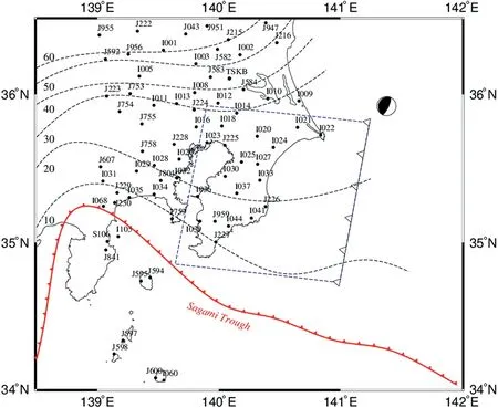
Fig. 2. The distribution of GPS stations and fault geometry in Boso, Japan (close-up view of the yellow rectangle area in Fig.1).Black dots indicate continuous GPS stations.The blue dot line is the surface projection of the rectangular fault plane. Red lines indicate the Sagami trough. Black dashed lines are iso-depth contours at 10 km intervals.

Table 1 The parameters of the fault sources offshore the Boso peninsula. Latitude and longitude indicate the positions of the upper right-hand edge of the rectangular fault.

3. Detection of SSEs using GPS data

3.1. GPS coordinate time series model

Surface continual GPS coordinate time series are modeled as the following equation [29]:

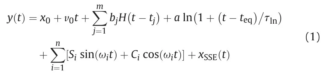
where y（t） is one component of GPS sites; t is the time in the decimal year;x0is the initial position;v0is the steady velocity;m is the number of coordinate steps with amplitude at the time of tj;H（t） is a step function; a is the amplitude coefficient of the logarithmic relaxation item;teqis the time of the large earthquake;τlnis the logarithmic relaxation time; Siand Cirelate to annual and semi-annual seasonal variations; ωi=2π/T (where T equals one year),n is the number of seasonal variations;xSSE（t）represents SSE time series containing the noise.

During the period from January 1, 2009 to January 1, 2011, the velocity v0is considered as the steady velocity of the site[38]. We repair the GPS coordinate time series steps based on the step file,referring to http://geodesy.unr.edu/NGLStationPages/steps.txt. The step files include the potential earthquake and equipment change from the IGS log file (antenna, receiver, or firmware change). The optimal values τlnare calculated using the nonlinear least square method.The estimated logarithmic relaxation time varies with GPS stations,is significantly related to the epicenter distance,and obeys the Gaussian distribution[39].The τlnvalues of the stations in the Boso peninsula are closed to 1 [39]. The order n in seasonal variation items is determined using the Akaike Bayesian information criteria(ABIC)[5].We use annual/semiannual sinusoidal curves and fit time series by the least square method to solve the sine/cosine functions[21].In the process of seasonal parameter estimation,we use data from the years in which non-slow slip occurs to avoid the influence of the past SSEs in extracting each SSE signal.Commonly,we could extract the signals of SSEs by modeling and removing the other signal sources.

3.2. Detection of Boso SSEs from 2011 to 2019

Examples of extracting SSE signals in Boso using GPS coordinate time series are shown in Fig. 3. From Fig. 3(a)-3(f), surface continual GPS coordinate time series are modeled using equation(1). The constant term, velocity term, step term, post-seismic logarithmic relaxation term, annual and semiannual periodic terms are removed, then we can extract SSE coordinate time series.Therefore, to obtain the signals of SSEs from GPS coordinate time series, it is necessary to perform data pre-processing and time series modeling.The basic process of extracting SSE signals from GPS time series is summarized as follows:(1)Calculating and removing the steps and gross errors in GPS time series (Fig. 3(a)); (2) Calculating and removing the secular velocity (Fig. 3(b)); (3) Modelling and removing the post-seismic relaxation item of the large earthquake (Fig. 3(c)); (4) Estimating and removing the seasonal variations (Fig. 3(d) and (e)).

The residual time series can ideally reveal and reflect the slow slip phenomenon after accurately modeling and correcting trend items, seasonal items, relaxation items, etc. Fig. 4 shows the extracted E/N/U residuals of the J266 GPS displacement time series in the Boso Peninsula from April 1, 2011 to January 1, 2019. Three SSEs can be observed in three durations,which are 5/15/2018-8/5/2018, 12/1/2013-1/31/2014, and 9/27/2011-12/25/2011, respectively.It is worth noting that a hidden SSE in March 2011,four days after the Tohoku earthquake,has been reported[40].However,we do not discuss this event because its small-amplitude signals might be masked by other noises.

In addition, the extracting SSE signals for the above basic process still contain other noises, particularly spatial-dependent common mode error (CME). CME may be present at all stations,which can be reduced by the spatial filtering method.Stacking and subsequent CME removal may alter the observed signal [21].Therefore, we use the principal component analysis (PCA) and stacking method [31,41] to analyze the influence of CME on Boso SSEs in section 4.2.

In Fig.3,the cyan dotted vertical line represents the time of the 2011 MW9.0 Tohoku earthquake.In Fig.3(a),the scattered blue dot represents the original GPS displacement time series from January 1, 2009 to April 1, 2019. The red vertical line represents the eliminated gross error and its error bar (error ratio magnified by ten times to facilitate clear display). The cyan vertical lines represent the repaired displacement steps. In Fig. 3(b), the scattered blue points represent the time series after removing the gross errors and repairing the steps, and the magenta diagonal lines indicate the constant and velocity terms.In Fig.3(c),the blue scatter points are the time series after the above pre-treatment steps in Fig.3(a)and(b), and the red logarithmic curve is the post-seismic logarithmic relaxation term caused by the 2011 MW9.0 Tohoku earthquake.The red harmonic lines in Fig. 3(d) and (e) represent the annual and semiannual periodic terms. In Fig. 3(f), the blue scatter points are the residuals after removing the constant term,velocity term,step term, post-seismic logarithmic relaxation term, annual and semiannual periodic terms,which contain the signals of SSEs and other noises.

4. Inversion of SSEs applying the PCAIM

4.1. Inversion method (PCAIM)

With the extracted SSEs time series from GPS data and the fault model built by the given fault parameters (Table 1), we use the PCAIM to resolve the slip distribution of SSEs in June 2018,December 2013-January 2014, and October-November 2011. The inversion process is briefly described as follows [22,42].

(1) Constructing matrix X0with the extracted SSE time series xSSE（t）. The rows of X0correspond to the coordinate components at GPS sites,and the column represents the SSE time series for a given period.

Fig. 3. Removal of gross error, steps, velocity, relaxation, annual and semiannual terms in GPS time series.

Fig.4. Extracted Boso slow slip time series from 2011 to 2019.The period between the two red vertical bars represents the test duration for the 2011 SSE.The period between the two green vertical bars represents the 2013-2014 SSE test duration. The period between the two magenta vertical bars represents the test duration for the 2018 SSE.

(2) Generating matrix X by centering X0, decomposing matrix X =USVtby using a standard singular decomposing method,and filtering X by defining Xr=UrSrVtrwith r principal components. U is the weighted principal slip distributions and V is the time function.

(3) Obtaining slip distributions Lrby inverting the left singular vectors G·Lr=Ur,where G denotes the Green functions.G is computed by the Okada model with a given fault geometry in section 2.2.

(4) Recombining matrix X≈Ur·Sr·Vtr≈G·Lr·Sr·Vtr.

These extracted GPS SSE time series during three test durations((a) 5/15/2018-8/5/2018, (b) 12/1/2013-1/31/2014, and (c) 9/27/2011-12/25/2011) are utilized as inputs to the PCAIM software in this study.We inverted the spatio-temporal slip distribution using GPS SSE coordinate time series from 77 GPS stations in Fig. 2 and the rectangular fault parameters in Table 1. Considering the shallowness of SSEs in the Boso region, we constrained the vertical depth of the fault on the Philippine Sea plate to within 30 km.

4.2. Principal component analysis (PCA)

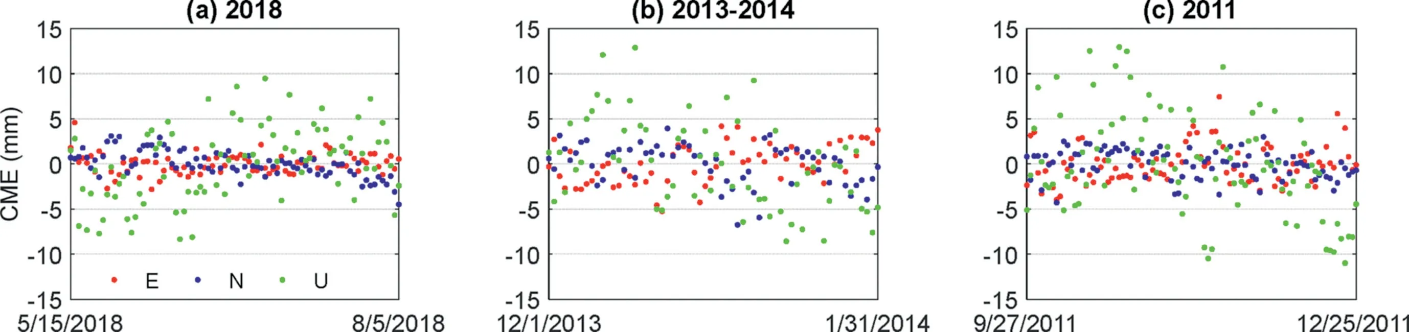
Fig. 5. Regional CMEs evaluated by stacking extracted GPS time series during three SSE test durations (a) 5/15/2018-8/5/2018, (b) 12/1/2013-1/31/2014, and (c) 9/27/2011-12/25/2011.

In this study, we evaluate the CMEs using the stacking method of GPS time series of several sites far away from the slip area(latitude ＞35.8°). The horizontal CMEs during the three SSEs are within 5 mm, and the CMEs in the U direction are within about 10 mm (Fig. 5). In addition, the PCA is utilized to estimate and extract the CMEs in GPS SSE coordinate time series. The PCA technique effectively reduces spatial and temporal CMEs.It helps to provide more accurate GPS SSE coordinate time series for detecting weak or transient signals [40]. The number of principal components in the PCA is determined according to the chi-square statistic value. The closer the chi-square value is to 1, the better the result[31]. In this test, suppose we use two principal components(Fig. 6(a) and (b)) instead of only one (Fig. 6(c)). The chi-square values show changes of no more than 0.1 as the number of principal components of SSEs increases in 2018, 2013-2014, and 2011.In that case,the first component is only statistically significant,and the slip of the second component is only a few mm. Therefore,subtracting the CMEs isolated by the stacking or PCA methods has little effect on Boso SSEs inversion. The number of the principal components is set to 1 in the SSE inversions with the PCAIM.

5. Spatio-temporal inversion analysis of SSEs

5.1. Surface displacement deformation

Fig. 7 shows the extracted SSE time series by GPS coordinate time series model and the computed surface displacement time series by PCAIM at selected I027 and I041 stations.Considering the differences between horizontal and vertical coordinate accuracy,we set the horizontal and vertical weights to 5:1 in the following analysis[30].The standard deviation in Fig.7 is estimated from the PCAIM inversion.The extracted SSE coordinate time series show an obvious transient signal in the E and N components. In Fig. 7,eastward and southward movements are observed at stations I027.During 6/6/2018-6/20/2018,12/30/2013-1/5/2014 and 10/23/2011-11/6/2011, we approximated the periods of detected SSEs. The periods and surface displacements of transients at I041 are similar to I027.

Fig. 8 shows the extracted and computed horizontal displacements of the 2018, 2013-2014, and 2011 SSEs. Their standard deviations are derived from the precision of GPS coordinate time series. We can see the extracted and computed horizontal displacements are consistent overall, suggesting that the inversion results from PCAIM are good.The displacement distributions of the three SSEs show obvious differences.The horizontal displacements of 2013-2014 SSE are significantly smaller than those of the other two SSEs. The 2018, 2013-2014, and 2011 SSEs all show southeastward movements, with the displacements of 5.3 cm, 1.7 cm,and 3.9 cm. The horizontal moving direction of SSEs is opposite to the moving direction of the Philippines plate,suggesting that SSEs occur on the plate interface. Furthermore, our results are in good agreement with the estimated displacement time series from Ozawa using the ENIF software [30].

5.2. Cumulative slip distribution and moment

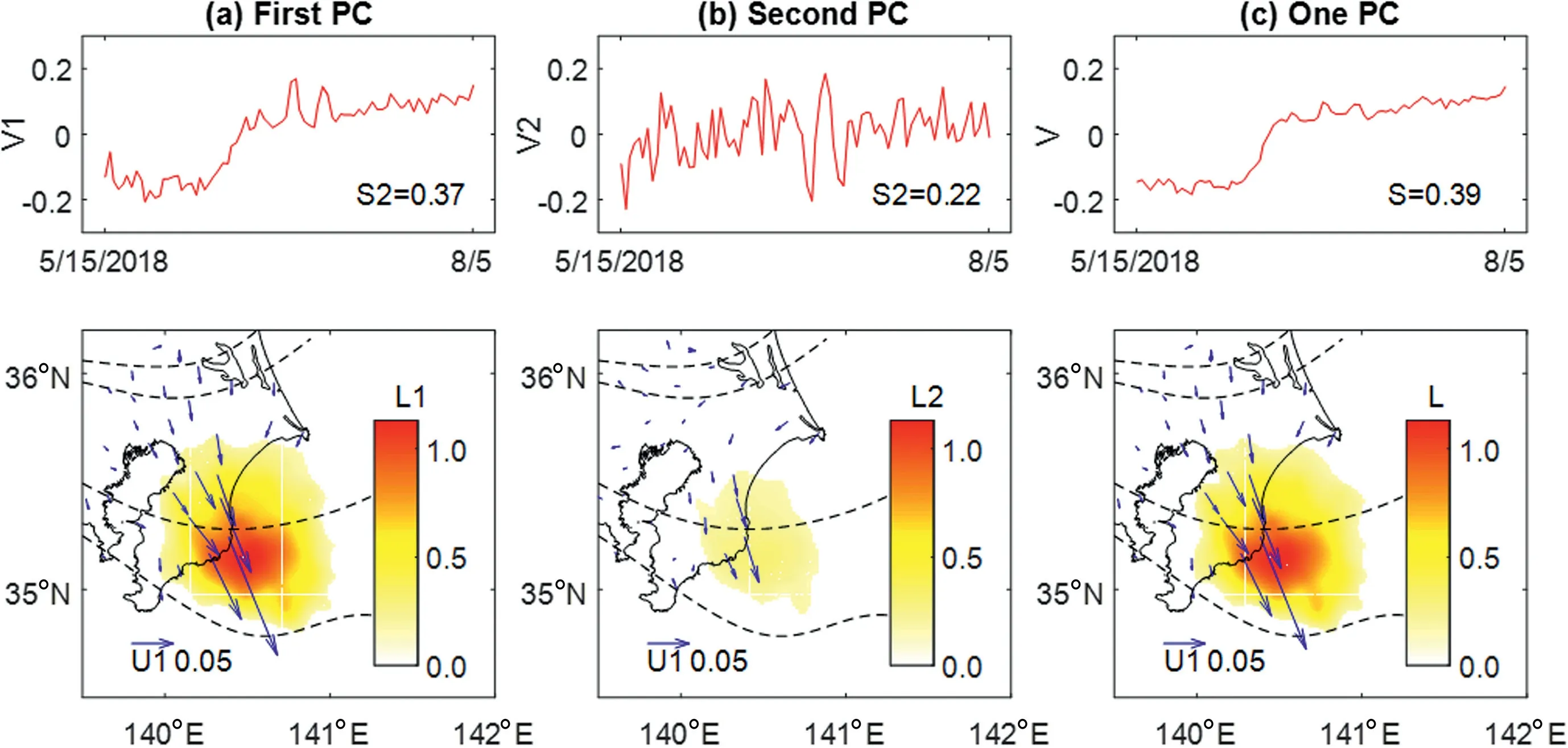
Fig.6. (a)and(b)indicate the first and second components by setting up two principal components.(c)corresponds to the only one PCA component by setting up one component.S is each principal component's weight (or contribution). V1, V2 and V represent the time functions. Blue arrows U1 represent the horizontal spatial distribution. The area marked with the hot color bar represents the slip distribution L on the fault surface.

Fig.7. The extracted SSE time series by GPS coordinate time series model and the computed displacements time series by PCAIM software at selected I027 and I041 stations,whose locations are shown in Fig.2.E,N,and U represent the three components of the east,north,and vertical components,respectively.Error bars represent the standard deviations.Red lines show the computed results from PCAIM, and the green vertical lines indicate the approximate start and end times of SSEs.

Fig.9 shows the cumulative slips of 2018,2013-2014,and 2011 SSEs,and the standard errors of the cumulative slips.The standard error can be used as a measure of uncertainty.In Fig.9(a),(b),and(c),we can see south-eastward movements of SSEs in the range of 10 km-25 km.The maximum cumulative slip is the slow slip of the 2018 SSE,which can reach 12.4 cm,followed by 9.2 cm of the 2011 SSE and 4.8 cm of the 2013-2014 SSE.Compared to Ozawa's studies[30], the cumulative slips of three SSEs are generally more minor,which might be due to the different extraction or inversion methods of the SSE time series. In Fig. 9 (d), (e), and (f), the maximum uncertainties are 0.5 mm, 0.5 mm, 0.3 mm for the inversions of 2018, 2013-2014, and 2011 SSEs. The uncertainty can not show the difference between the calculated results and the truth value, but it can be used to compare the calculated results.The smaller the uncertainty, the higher the precision of the calculated results.In our study with the same parameters configuration,the precision and SNR of the extracted GPS SSE time series may be the main factors affecting the uncertainty of SSE's inversion.Three areas where the SSEs occur are almost the same, located in the southeast of the Boso peninsula,but the depth of 2013-2014 SSE is 5 km deeper than that of 2018 and 2011 SSEs. The maximum cumulative slips of the 2018 and 2011 SSEs occur at depths between 15 km and 18 km,and the maximum cumulative slip of 2013-2014 SSE occurs at about 20 km.The location of the central area is almost consistent with Fukuda's research on 2013-2014 SSE[28]but 5 km deeper than that of Ozawa's studies on 2018 SSE [30].

Fig.10 shows the time evolution of the estimated moment of the 2018,2013-2014,and 2011 SSEs.The moments are calculated from the estimated slip, with the rigidity of 30 GPa. The total released moments of the SSEs are 13.1 × 1018N·m (MW6.7) in 2018,6.2 × 1018N·m (MW6.4) in 2013-2014, and 10.6 × 1018N·m(MW6.6). According to the moment release, the approximate durations of 2018, 2013-2014, and 2011 SSEs are two weeks, one week, and two weeks, respectively, which are similar to the detected SSE time series durations.

Table 2 summarizes the three SSEs inversion results containing the maximum cumulative slips and seismic moments of the indicated test duration.Furthermore,the 2013-2014 SSE showed minor seismic moment MW6.4 than the 2011 MW6.6 and 2018 MW6.7 SSEs, which may be correlated with the nucleation style[29]. Gardonio proposed that the moment magnitudes of these SSEs are between 6.4 and 6.6[34],which is similar to our research results.Table 2 also shows the approximated periods for detected three SSEs from the displacement time series. Even if we have detected and inverted the three SSEs, the understanding of the temporal and spatial evolution of SSEs is still limited. Thus, to further analyze the three SSEs,we carry out the detailed temporal and spatial evolution of SSEs,which is helpful for us in identifying SSE nucleation.

Fig.8. Total south-eastward transients for 2018,2013-2014,and 2011 SSEs.Blue arrows represent horizontal displacements for SSEs,while red arrows represent computed results from PCAIM. Green error ellipses show horizontal displacement accuracies.

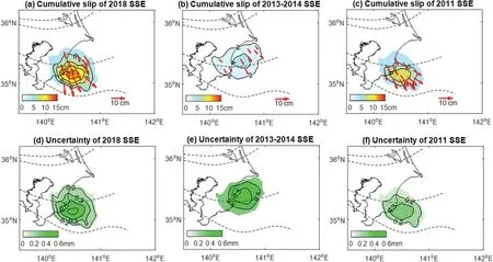
Fig.9. (a),(b),and(c)represent the cumulative slip distributions of the 2018,2013-2014,and 2011 SSEs.The color indicates the size of the slip,the contour intervals are 2 cm,and the solid arrows indicate the slip's direction in(a),(b),and(c).(d),(e),and(f)represent the uncertainties of the cumulative slips of the 2018,2013-2014,and 2011 SSEs,in which the color indicates the size of the uncertainty, and the contour intervals are 0.1 mm.

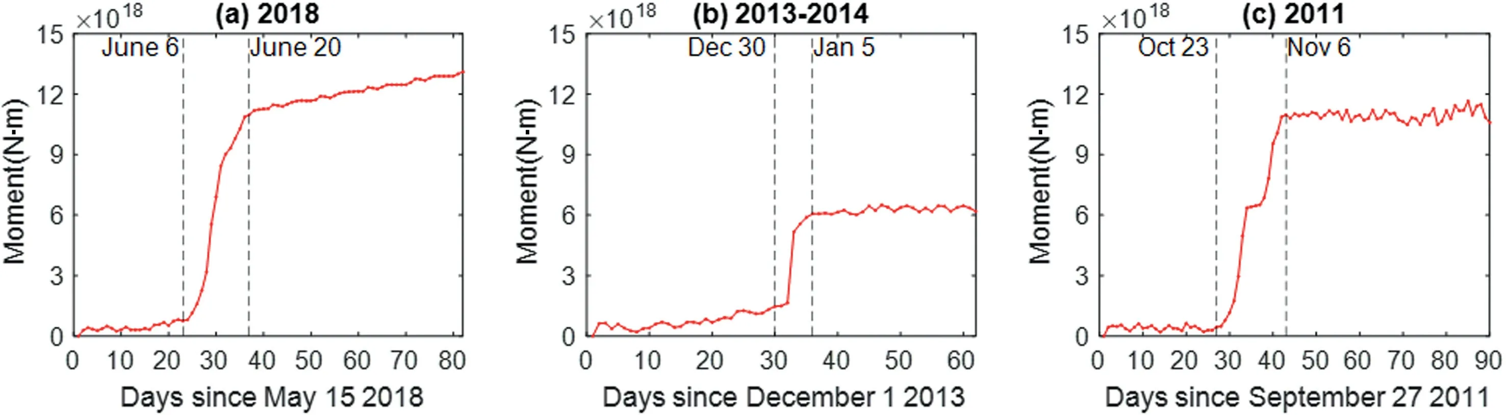
Fig.10. (a),(b),and(c)represent the cumulative moment release of the 2018,2013-2014,and 2011 SSEs.The vertical dashed lines indicate the approximate beginning and end of the SSEs.

5.3. Spatio-temporal evolution history

Figs.11-13 show the spatio-temporal evolutions of SSEs per 2 days estimated by PCAIM.We evaluate the slip from the start to the end of the transient deformations,including the significant changes of 1-2 weeks. Combining the 2018 SSE coordinate time series(Fig.7)and slip evolution(Fig.11),we recognize that the 2018 SSE began on June 6,2018,offshore eastern side of the Boso Peninsula,and accelerated to June 14, with the maximum slip rate reaching 2.1 cm/day. During the slip acceleration phase in the first week of 2018 SSE, the center of the slip area does not change, but the slip zone expands.During the second week from June 14 to June 20,the slip area shrinks back, the slip rate drops from June 16-18 to June 18-20, and nearly disappears.As shown in Fig.12,the 2013-2014 SSE experiences an acceleration period from December 30,2013 to January 3, 2014, and then rapidly decelerates until January 5. The maximum slip rate of 2013-2014 SSE is 1.3 cm/day,close to 1.1 cm/day calculated by Ozawa using ENIF [30]. Fig.13 shows the spacetime evolution of 2011 SSE. There are two phases of the slow slip in 2011, the first phase is from October 23 to October 31, and the second phase is from November 2 to November 6. The maximum slip rate in the first stage reached 1.8 cm/day.During 2018(Fig.11),2013-2014(Fig.12)and 2011 SSEs(Fig.13),the slip zone expands in the acceleration phase of slip, and it shrinks back in the deceleration phase of slip. Compared with 2013-2014 and 2018 SSEs, the 2011 SSE shows a different and more discontinuous expansion behavior.Fukuda proved that earthquakes continued to migrate in the direction of sliding extension at similar slow slip speeds in 2011 and 2013-2014 [29]. Therefore, the slip expansions of the three SSEs are different, but there are no apparent spreads in the center area of the slip in each SSE.

Table 2 The period, MW, maximum slip of the 2018,2013-2014, and 2011 SSEs.

Fig.12. Spatio-temporal evolution history of the 2013-2014 SSE.

Fig.13. Spatio-temporal evolution history of the 2011 SSE.

The analyses of the spatio-temporal evolution of slip reveal that the nucleation styles of 2018, 2013-2014, and 2011 SSEs are different.The 2013-2014 SSE exhibits more rapid time changes but shows deeper slip, shorter slip duration, minor seismic moment,and lower slip rate. The 2018 SSE shows the most significant seismic moment,maximum slip,and slip rate.The overall evolution of the SSEs suggests that the nucleation of the 2011 SSE is the most complex involving two processes.The nucleation styles of 2018 and 2013-2014 SSEs are similar, and the 2013-2014 SSE nucleated more rapidly.

6. Discussion and conclusion

The previous studies show that the Boso SSEs begin to accelerate and last for 1-2 weeks [26,28,43,44]. The durations of the significant transient slip deformation phase in our study are generally consistent with these previous studies. However, there are still substantial differences between 2018, 2013-2014, and 2011 SSEs.The 2011 and 2018 SSEs are about two weeks, but the 2013-2014 SSE just last about one week. In addition, the slip rates of 2018,2013-2014, and 2011 SSEs change in different ways. In particular,the evolution of 2011 SSE is divided into two distinct acceleration and deceleration phases, while there is only one acceleration and deceleration phase in 2018 and 2013-2014 SSEs, and the acceleration and deceleration of 2018 SSE are slower. Furthermore, the seismic moment,the maximum slip,and the maximum slip rate are minor using the PCAIM in our study than those using the ENIF method in Ozawa's study[30].The slip is about 5 km deeper in the PCAIM model than that in the ENIF model. Even though the inversion of the SSEs using different methods has some differences,the spatio-temporal variation trends of the three SSEs are almost relatively consistent.

In addition, a recurrence interval of 4-7 years is identified in 1983, 1990, 1996, 2002, and 2007 before the 2011 Tohoku earthquake [29,30]. However, our study shows that the recurrence interval has changed from 2.2 to 4 years from 2011 to 2019. The recurrence intervals in 2007, 2011, and 2013-2014 are shorter because of the 2011 MW9.0 earthquake [34]. Numerical friction models indicate that the recurrence interval of SSEs may be shortened when a large inter-plate earthquake is about to occur nearby [34]. After the 2013-2014 SSE, the period of the SSE gradually returns to normal. According to the periodicity of Boso SSEs,the future SSE is likely to occur 4-7 years after the 2018 SSE if there is no large earthquake.

This study shows the detection and spatio-temporal evolution of the Boso 2018, 2013-2014, and 2011 SSEs using GPS data and the PCAIM. We first extracted the SSE displacement time series from GPS data by modeling and reducing the influence of postearthquake deformation, steady deformation, seasonal variations,and other time-dependent errors, which is critical for detecting slow slip events. Then, a fault model was constructed to approximate the actual crustal structure at the Boso region using a point source model in a homogenous elastic half-space. Finally, we used the PCAIM to retrieve the spatio-temporal distribution of the SSEs.The results indicate that the 2018 SSE has the largest total movement and the most significant slip, and the 2013-2014 SSE has a significantly shorter duration and smaller surface displacement.The 2011 SSE shows a more discontinuous expansion phenomenon.The spatio-temporal evolution of the SSEs reflects the nucleation style, suggesting that the nucleation of 2011 SSE is the most complex involving two processes, while the nucleation styles of 2018 and 2013-2014 SSEs are almost the same,and the 2013-2014 SSE nucleated more rapidly.

Conflicts of interest

The authors declare that there is no conflicts of interest.

Acknowledgments

The GNSS time series products are available from the Nevada Geodetic Laboratory archive (http://geodesy.unr.edu). A software package, Generic Mapping Tool (GMT) (Wessel and Smith, 1998),was used to plot Figs.1 and 2. We thank the California Institute of Technology for the PCAIM inversion software. This research was funded by the National Natural Science Foundation of China(41704031, 41904015, 42061077); the Young People Science Foundation of Jiangxi Science and Technology Department(20192BAB217011); the open fund from Engineering Research Center for Seismic Disaster Prevention and Engineering Geological Disaster Detection of Jiangxi Province(SDGD202109).We value the assistance of the reviewers and the Editorial Office of Geodesy and Geodynamics to better the manuscript.