Fault Diagnosis Method Based on Xgboost and LR Fusion Model under Data Imbalance

Liling Ma, Tianyi Wang, Xiaoran Liu, Junzheng Wang, Wei Shen

Abstract: Diagnosis methods based on machine learning and deep learning are widely used in the field of motor fault diagnosis. However, due to the fact that the data imbalance caused by the high cost of obtaining fault data will lead to insufficient generalization performance of the diagnosis method. In response to this problem, a motor fault monitoring system is proposed, which includes a fault diagnosis method (Xgb_LR) based on the optimized gradient boosting decision tree(Xgboost) and logistic regression (LR) fusion model and a data augmentation method named data simulation neighborhood interpolation(DSNI). The Xgb_LR method combines the advantages of the two models and has positive adaptability to imbalanced data. Simultaneously, the DSNI method can be used as an auxiliary method of the diagnosis method to reduce the impact of data imbalance by expanding the original data (signal). Simulation experiments verify the effectiveness of the proposed methods.

Keywords: imbalanced data; fault diagnosis; data augmentation method

1 Introduction

Fault diagnosis plays an important role in the normal operation of the motor [1]. With the rapid development of machine learning, a large number of machine learning models are used in the field of fault diagnosis [2, 3]. Generally, these models can be abstracted into a structure like“feature extraction + classifier”. The advantage of this data-driven diagnosis method is that it does not require a clear or complete system model, but its performance depends mainly on the number and quality of features and the structure of the classifier [4]. Commonly used diagnosis method classifiers are logistic regression [5,6],decision tree [7], support vector machine [8], artificial neural network [9], hidden Markov model[10].

Recently, convolutional neural networks(CNN) are applied to the field of fault diagnosis.Yu et al. used Fourier transform to obtain the signal’s spectrogram and perform fault diagnosis through image recognition [11]. V. David et al.proposed to convert the input of a convolutional neural network into a time-frequency map obtained by short-time Fourier transform [12].Guo used the continuous wavelet transform scale map as a feature [13]. Instead of converting the time domain data to the frequency domain, the sampling values of the signals were intercepted in time sequence, and multiple one-dimensional sampling signals were spliced together in time sequence to form a two-dimensional feature map[14]. Ince et al. adjusted the structure of the convolutional neural network and replaced the twodimensional convolution kernel with a one-dimensional convolution kernel. The one-dimensional convolutional neural network was applied in motor fault diagnosis, which directly accepts the original data (signal) as input [15].

Although these methods have satisfactory accuracy in detection, in practical situations, the acquisition cost of motor fault data is high. During most of the operation, the machine is running in a healthy scenario, and in fact, effective error data is rare. It will lead to serious data imbalance problems and will directly affect the diagnosis accuracy of most methods [16]. In principle, most methods are optimized based on the loss function. Data imbalance will cause the gradient iteration of most classes to dominate during optimization. The intuitive recognition is that the classifier tends to divide the data into majority classes to maintain a proper diagnosis accuracy. At present, the main method is to reduce the impact of data imbalance from the model and the data. On the one hand, the models that are less sensitive for data imbalances are used, such as the tree model [17], SVM [18]. On the other hand, the data set is balanced by sampling data or data augmentation methods based on the vicinal risk minimization principle(VRM) [19]. Taking image processing as an example, common sampling methods include undersampling [20]and oversampling [21]. A typical data augmentation strategy is to use horizontal reflection, rotation, scaling, and noise addition [22]. Mao et al.developed a method for initial fault diagnosis of high-speed train traction system based on stacking generalization with Xgboost as the estimator in the first layer of the stack and logistic regression (LR) as the estimator in the second layer[23]. Zhang et al. proposed a WMODA algorithm combining weighted minority oversampling (WMO) and the enhanced deep autoencoder (DA) method. Compared with traditional data-driven methods, WMODA can detect more fault samples in fault detection of imbalanced data [24]. However, the sampling and augmentation methods for industrial signals are still being explored.

In this paper, a motor fault monitoring system is proposed, which includes a fault diagnosis method (Xgb_LR) based on the optimized gradient boosting decision tree (Xgboost) and logistic regression (LR) fusion model and a data augmentation method named data simulation neighborhood interpolation (DSNI). The proposed Xgb_LR diagnosis method has the advantages of fast response speed, high universality, and strong adaptability to data imbalance. Xgboost is used to automatically obtain combined features and adapt to data imbalance to improve the learning ability of the logistic regression model. The proposed DSNI method is used to expand the original signal data set to adjust the balance of the data set. It is based on the idea of autoencoder,using Fourier transform FFT and principal component analysis PCA and their inverse transform to replace encoder and decoder section. It can be used as an auxiliary method of fault diagnosis method to reduce the impact of data imbalance. The proposed method is stable and efficient, and can be used as the main diagnosis method for a fast and accurate real-time motor fault monitoring system.

The rest of this article is organized as follows: The Xgb_LR algorithm and the DSNI method are illustrated in detail in Section 2. In Section 3, the proposed methods are verified by simulation experiments, including data set acquisition and analysis of results. Finally, Section 4 concludes the paper.

2 The Proposed System

2.1 Fault Diagnosis Method Based on Xgb_LR

2.1.1 Overview of Xgboost

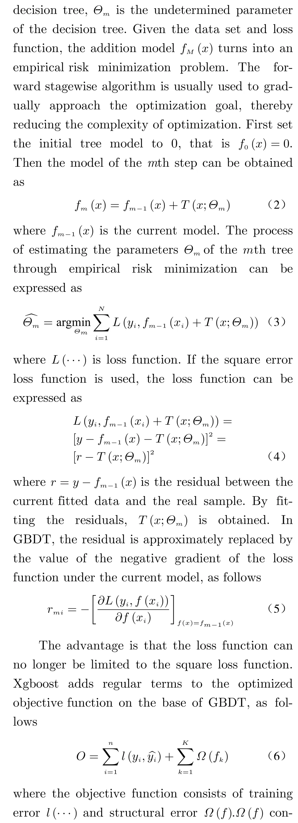
Xgboost is a kind of optimized gradient boosting decision tree (GBDT). GBDT is an integrated learning method based on the boosting idea. By using the CART decision tree as the base classifier, the weak learners are promoted to strong learners. The boosting tree can be described as an additional model of decision trees as

2.1.2 Xgb_LR Fusion Model In this paper, a motor fault diagnosis model named “Xgb_LR” based on the fusion model of Xgboost and LR is proposed. First, the threephase current of the stator of the motor is collected. Next, fast Fourier transform(FFT) is used to extract features from the collected data,and the features are inputted into the Xgb_LR model for fault diagnosis. In Xgb_LR, the datasetDis used to construct the gradient boosting decision tree Xgboost. Then the leaf node number of each sample inDfalling in the tree is taken as the second feature of each sample. The leaf node number is encoded by one-hot, and the encoded result is used as the input of the logistic regression (LR) model. LR is used to learn the weights of these new feature combinations. Fig. 1 illustrates the schematic diagram of the Xgb_LR model.

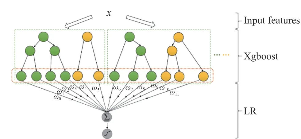
Fig. 1 Xgb_LR model

A strategy named “One vs Rest” (OVR) is used to implement multi-category diagnostic tasks. For a diagnosis task withNscenarios, one of the scenarios is taken as a positive example and the rest are negative examples. Then a tree is trained using the reconstructed data set; Each scenario is traversed as a positive example, and a new round of iteration is performed after trainingNtrees. After the training is completed, the number of each sample falling into the leaf node is encoded by one-hot. The coded number is inputted into the LR model as a secondary feature. The specific process is summarized as Algorithm 1.

Algorithm 1 Xgb_LR algorithm process Input:1. Data set D;2. Number of status categories N;3. Number of iterations t;Output:4. Xgb_LR Model 5. for i = 1 to t do 6. for j = 1 to N do 7. Generate a tree jij;8. end for 9. end for 10. Collect the leaf node number of the tree which the data falls into, and implement one-hot encoding;11. Use the processed features as input to LR model.

12. Obtain Xgb_LR model;

2.2 Data Simulation by Neighborhood Interpolation

According to the VRM principle, the general idea of data augmentation is to use a priori knowledge to describe the neighborhood of each sample in the training data, and then interpolate in the field of training samples to generate virtual samples. It is difficult to describe the neighborhood of the current signal from a time domain.Because the amplitude of the current will change when the motor is in different fault scenarios.The sample neighborhood divided by amplitude is likely to contain samples of different scenarios.The autoencoder provides an indirect way to determine the neighborhood of the sample. Fig. 2 manifests a simple autoencoder. The autoencoder first compresses the input into a latent representation through the encoder section, as follows

Fig. 2 A simple autoencoder

The autoencoder makes the reconstructed outputrto be as close as possible to the original inputxso that the latent representationhcan uniquely represent the original input. By operating on the latent representationh, a virtual sample can be generated forhindirectly according to the VRM principle. Then through decoder reconstruction, the generated samples are obtained that are similar to the inputxbut not the same.Based on this indirect generation idea, a timedomain data augmentation method named data simulation neighborhood interpolation (DSNI) is proposed.to generate a virtual latent representation, wherecrepresents the amount of data augmentation,rand(0,1)is random number between (0, 1).Then, the obtainedh*newis decoded by the inverse transform of PCA and FFT, and the reconstructed output is the generated virtual sample.The label of the new sample is consistent withxi.The whole process is shown in Fig. 4, and the procedures are summarized as Algorithm 2.

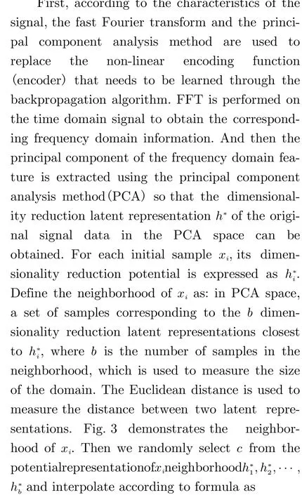
Fig. 3 The neighborhood of xi

Algorithm 2 DSNI Algorithm Input:1. Data set D 2. Neighborhood size b;3. Number of data augmentation c.Output:4. Augmented data set Daug 5. Calculate the FFT result DF of D by FFT;6. Calculate the PCA result DP of DF by PCA, principal component matrix is denoted as Uk;7. For each data (d) in data set DP, calculate the Euclidean distance from other data which belong to the same category, and take the first b samples of the closest distance to form a neighborhood;8. Randomly select c samples from the neighborhood and calculate according to equation (13) to obtain the latent representation of the new sample ;dF h*aug aug h*aug UTk 9. Calculate the iPCA result of by ;daug dF 10. Calculate the iFFT result of by iFFT;daug Daug 11. Collect the obtained into a collection .aug

Fig. 4 DSNI algorithm process

3 Simulation Experiments

3.1 Data Sets and Experiment Settings

The permanent magnet synchronous motor is taken as the research object. Some parameters of the motor are as follows: rated output power 750 W, rated speed 3 000 r/min, rated phase current 4.78 A, instantaneous maximum phase current 14.4 A. First of all, the motor current signals are collected in the order of A phase, B phase, and C phase, and combined with the given label to form a data set. In each simulation experiment, the current signal collects 128 points per cycle. The motor is controlled to run in the range of 0–3 000 r/min, and then the fault and the time when the fault occurs are set. Starting from the first two cycles of the fault, the threephase current data of 4.5 cycles is collected backward every other cycle, and combined as the data in the order of A-B-C, so that the characteristics of the three phases can be integrated. Repeating the above process, a data setDTis formed by one-to-one correspondence between the obtained data and the labels. Healthy, permanent magnet demagnetization failure, A phase to ground short circuit failure, A phase and B phase short circuit failure is taken as the research object. 200 data of each scenario are taken fromDTto form the data setD.

In the experiment, a variety of classic machine learning fault diagnosis algorithms are trained and tested. The implementation details are described in Tab. 1. Fig. 5 illustrates the block diagram of the fault diagnosis algorithm.

Tab. 1 Fault diagnosis accuracy on four scenarios %

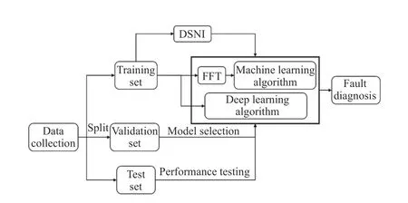
Fig. 5 Block diagram of fault diagnosis method

To simulate a terrible situation, half of the data from data setDare randomly selected to form data setDfew. First, DSNI algorithm is executed on the data setDfewto obtain the augmented data setDaug. Next, these two data sets are used to train and test machine learning fault diagnosis methods and deep learning fault diagnosis methods. Finally, we set the imbalance as 1: 3 to simulate the imbalance under a few-shot.120 health scenario time-domain data and 30 demagnetization fault data are randomly selected to form a data setDub. The demagnetization fault data are expanded 3 times by the DSNI algorithm. Then the expanded data is combined with the original data setDubto form a balanced data setDb. These two data sets are used for comparative experiments to verify the effectiveness of the proposed method.

3.2 Results and Analysis

3.2.1 Xgb_LR Performance Verification

The fault diagnosis results of the four scenarios are manifested in Tab. 1, where “0” is healthy,“1” is permanent magnet demagnetization failure, “2” is A phase to ground short circuit failure, “3” is A phase and B phase short circuit failure. Several repeatable experiments are conducted to calculate the average diagnosis accuracy of the four scenarios. From Tab. 1, the diagnosis effect of the method using model fusion is better than the method using a single model.From a computational perspective, diagnosis algorithms tend to fall into the local minimum.Model fusion can reduce the risk of getting into a bad local minimum point, thus making the model more stable; In terms of representation, the single diagnostic algorithm has limited representation space. Through model fusion, the hypothesis space can be expanded, and it is possible to learn a better approximation; From a statistical point of view, there may be multiple hypothetical models with similar performance on the training set. Model fusion can reduce the risk of poor generalization caused by single learner misselection. Meanwhile, using the LR model with a simpler structure can reduce the overfitting effect brought by the tree model, and can improve the generalization performance.

From the perspective of feature engineering,GBDT provides a variety of feature combination methods for logistic regression, as shown in Fig. 6. A series of feature combinations can be obtained from each leaf node of the decision tree back to the root node. Encoding data through Xgboost is equivalent to introducing a variety of high-order features, which improves the nonlinear expression ability of the model to a certain extent. In the meantime, Xgboost goes further than GBDT by leading regular terms into the objective function. In terms of the perspective of the deviation-variance, the regular term reduces the variance of the model, which makes the model simpler, and effectively prevents overfitting, thereby improving the diagnosis performance of the method.

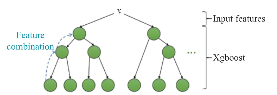
Fig. 6 Feature combination by Xgboost

Tab. 2, Fig. 7 and Fig. 8 show the average training time and fault diagnosis time of the fault diagnosis method. The Xgb_LR model takes more training time than the GBDT model. It is because although Xgboost uses parallel processing to reduce training time, it uses the second derivative of the loss function when optimizing.The calculation of the Hessian matrix related to the second derivative is extremely time-consuming. However, the advantage of using the second derivative is obvious, which allows the model to converge faster. When the first and second derivatives of the loss function are guaranteed to exist, the loss function can be customized. Compared with the logistic regression model, the fusion model significantly improves the diagnosis accuracy, but also pays several times the time overhead. However, it is obvious that the time spent in this part is insignificant compared to the time spent manually performing feature combinations. The advantage of the diagnosis method based on the LR model over the SVM model is the diagnosis speed. Although SVM derives the concept of support vectors, which greatly reduces the training time, due to the existence of kernel functions, it leads to greater computational complexity in the diagnosis process.

Tab. 2 Average running time

Fig. 7 Average training time

Fig. 8 Average diagnosis time

The proposed Xgb_LR method has a good balance between running time and diagnosis accuracy, which not only ensures the efficiency of the diagnosis process but also takes into account the real-time diagnosis.

Fig. 9 demonstrates the receiver operating characteristic curve (ROC) in the case of two scenarios (healthy/demagnetization failure). The abscissa is the false positive rate and the ordinate is the true positive rate. Xgb_LR fault diagnosis method has the largest area under curve (AUC), which means its performance is better than other models. Especially in the area of high sensitivity and high specificity (the upper left of the ROC), Xgb_LR has the best performance. It means that the method is less prone to missed detections and misdiagnose, and is more in line with the basic requirements of fault diagnosis.

Fig. 9 ROC for healthy and demagnetization failure

3.2.2 DSNI Performance Verification Principal component analysis (PCA) is used to visualize the data set. After extracting features from the data setDthrough FFT, the first 20-dimensional data under PCA can express 97.53%of the original data information. Fig. 10 illustrates the distribution of the first three dimensions of the datasetDunder PCA. It can be intuitively seen that through data enhancement, the diversity of data is expanded to a certain extent,and the information of the data set is enriched. A certain sample is randomly selected to execute DSNI method, and its time-domain diagram is shown in Fig. 11. It can be seen that the data extended by DSNI is safer in the time domain,and the data label will not change due to the sudden change in amplitude.

The original small sample data setDfewand the expanded data setDaugare used to train and test a variety of methods. Tab. 3 illustrates the experimental results. It can be clearly seen that after data augmentation, the accuracy of various diagnosis methods has increased to some degree.First, the DSNI method reduces the structural risk of the model by expanding the data set and brings a certain regularization effect. Second, performing neighborhood interpolation in the dimensionality reduction space in the frequency domain is equivalent to introducing some noise in the time domain to a certain extent. Using such data sets to train models can improve the stability and robustness of diagnosis methods. Third, the DSNI method uses FFT and PCA and the corresponding inverse transform to replace the encoding and decoding section of the autoencoder structure, so that the method obtains a certain degree of interpretability. Manipulating the frequency spectrum of the signal is in line with the intuitive understanding of the signal. Fourth, in a strict sense, the DSNI method is to generate a virtual sample in the neighborhood of the latent representationhthrough the oversampling method SMOTE. It will lead to a certain amount of overfitting, so diagnosis methods need to deal with overfitting to reduce variance.

Fig. 10 Data visualization(first 3 dimensions): (a) original data distribution; (b) data augmentation distribution

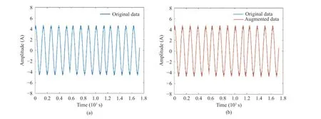
Fig. 11 Time domain graph: (a) original data; (b) data augmentation

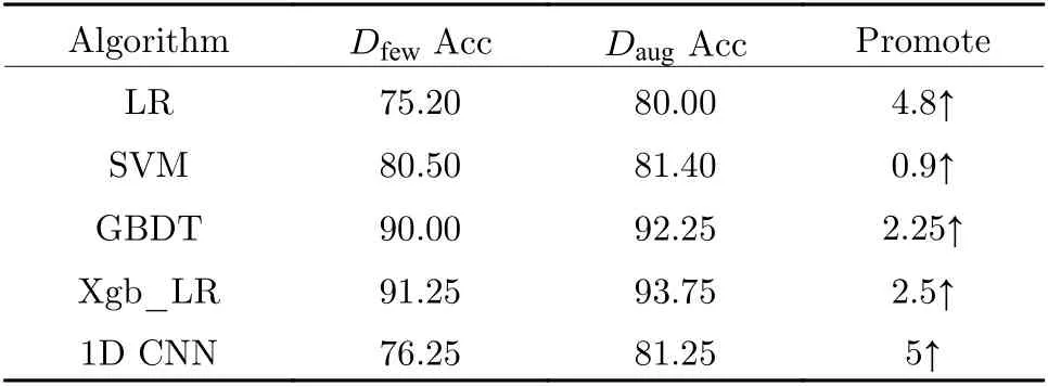
Tab. 3 Diagnosis accuracy before and after data augmentation %

It can be seen from Tab. 3 that DSNI has the most significant improvement effect on the one-dimensional convolutional neural networks diagnosis method (1D CNN). CNN has a strong learning ability and assumes a large space. Fewshot makes the model not fully trained. The DSNI method reduces the adverse effects of small samples to some degree, but the data diversity introduced is limited. For the diagnosis method based on SVM, the improvement effect of the DSNI method is not obvious. It is because the SVM uses the hinge loss function and derives the concept of support vectors. The hyperplane used for the boundary only depends on the support vector and has nothing to do with other samples.The DSNI method cannot significantly expand the number of support vectors, so the effect of improving SVM is not obvious. On the other hand, it can be verified that the proposed Xgb_LR method is more adaptable to few-shot and has higher diagnosis accuracy.

In the simulation experiment of data imbalance, use the data setsDubandDbto train the same fault diagnosis method respectively. Tab. 3 illustrates the results. It can be obviously seen from Tab. 4 that the serious data imbalance makes various diagnostic methods have reduced diagnosis accuracy, especially for the diagnosis method composed of a single learner. After the implementation of DSNI, various diagnostic methods have significantly improved accuracy. In the case of data imbalance, diagnosis methods based on loss function optimization and gradient descent updating parameters (such as LR, CNN)will incline the model to most classes, resulting in a decline in the generalization performance of the model, due to the small number of samples in the minority class-leading to insufficient gradient update. The model has reached the convergence condition before fully fitting the negative samples. However, the updating and optimizing strategies of diagnosis methods based on decision trees are different. The CART tree selects the divided features by the information gain of the features to make the samples of each node more“pure” so that the samples can be forcibly distinguished. Even if there is an imbalance in the number of data samples, the model will give sufficient attention to the minority class. Therefore,in the case of imbalanced data, the tree model will obtain more ideal generalization performance. Based on the above analysis, it can be seen that the proposed DSNI has a significant improvement effect on data imbalance, and the proposed Xgb_LR model has positive adaptability and generalization to imbalanced data.

Tab. 4 Diagnosis accuracy of imbalance experiment (%)

4 Conclusion

In this paper, a fault diagnosis system is proposed which includes Xgb_LR fault diagnosis algorithm and DSNI data augmentation method to reduce the impact of data imbalance and fewshot problems caused by the difficulty of obtaining motor faults in the actual process. The proposed Xgb_LR diagnosis method has certain adaptability to data imbalance and maintains high fault detection accuracy under the condition of few-shot. The proposed DSNI method based on the VRM principle generates virtual samples by interpolating in the field of latent representation, thereby expanding the diversity of data to a certain extent. As an auxiliary method of fault diagnosis method, DSNI obviously improves the performance of the diagnosis method under the conditions of data imbalance and few-shot.

The proposed methods have been tested with simulated data. The results of experiments prove the potential and effectiveness of the Xgb_LR method as a fault diagnosis method for real-time permanent magnet synchronous motors. It takes into account the high efficiency of the diagnosis results and the rapidity of the diagnosis process and has good prospects for use. Meanwhile, it is verified by simulation experiments that the proposed DSNI method has a positive auxiliary effect on a variety of fault diagnosis methods,especially for methods based on one-dimensional Convolution Neural Network. It can reduce the adverse effects caused by data imbalance and few-shot to a certain extent. In the future, we hope to study the data generation methods and generalization methods based on deep learning and apply them together with the DSNI method in the real-time monitoring of actual motor systems.